import matplotlib
if not hasattr(matplotlib.RcParams, "_get"):
    matplotlib.RcParams._get = dict.get

(Optional) DDIM (Denoising Diffusion Implicit Models): From the DDPM Perspective

About Me Publications My Teaching Research Notes

---

Once Loop Reflect

This notebook assumes you already understand DDPMs well, including:

• the forward diffusion process

• the closed-form marginal \(q(x_t \mid x_0)\)

• the posterior \(q(x_{t-1}\mid x_t, x_0)\)

• the learned reverse model \(p_\theta(x_{t-1}\mid x_t)\)

• ELBO training

• \(\epsilon\)-prediction, \(x_0\)-prediction, and \(v\)-prediction

• ancestral sampling

The goal here is to study DDIM rigorously and carefully as a new sampler built on top of the DDPM training setup.

We will keep notation consistent with standard DDPM notation:

• \(x_0\): clean sample

• \(x_t\): noisy sample at timestep \(t\)

• \(\alpha_t = 1 - \beta_t\)

• \(\bar\alpha_t = \prod_{s=1}^t \alpha_s\)

• \(\epsilon_\theta(x_t,t)\): model-predicted noise

• \(\hat x_0\): reconstructed clean sample estimate

• \(v_\theta(x_t,t)\): velocity prediction, when used

The notebook is structured as a technical tutorial:

1. prerequisites beyond DDPM

2. DDPM sampling recap

3. DDIM intuition

4. DDIM derivation

5. deterministic vs stochastic DDIM

6. timestep sub-sampling

7. classifier guidance

8. classifier-free guidance

9. implementation notes

10. common confusions

11. summary and comparison

Show code cell source

Hide code cell source

import numpy as np
import matplotlib.pyplot as plt

plt.rcParams["figure.figsize"] = (8, 5)
plt.rcParams["axes.grid"] = True
plt.rcParams["font.size"] = 11

Prerequisites Beyond DDPM

To understand DDIM properly, we need a few ideas beyond standard DDPM derivations.

1. What part of DDPM sampling is stochastic?

In ancestral DDPM sampling, the reverse transition is Gaussian:

\[ p_\theta(x_{t-1}\mid x_t) = \mathcal N\!\big(\mu_\theta(x_t,t), \Sigma_\theta(x_t,t)\big). \]

In the common scalar-variance case,

\[ \Sigma_\theta(x_t,t) = \sigma_t^2 I, \]

so one reverse step is

\[ x_{t-1} = \mu_\theta(x_t,t) + \sigma_t z, \qquad z \sim \mathcal N(0,I). \]

Thus the fresh Gaussian term \(\sigma_t z\) is the explicit source of stochasticity during reverse sampling.

---

2. What quantity determines randomness?

The amount of randomness is controlled by the reverse variance:

\[ \sigma_t^2. \]

In standard DDPM ancestral sampling, this is typically chosen as the posterior variance

\[ \tilde\beta_t = \frac{1-\bar\alpha_{t-1}}{1-\bar\alpha_t}\beta_t. \]

So the reverse randomness at each step is determined by the scale of \(\sigma_t\).

---

3. Deterministic vs stochastic trajectories

A reverse generative trajectory is the chain

\[ x_T \to x_{T-1} \to \cdots \to x_0. \]

• If every step includes fresh noise, the trajectory is stochastic.

• If no fresh noise is added, the trajectory is deterministic once \(x_T\) is fixed.

DDIM will let us continuously interpolate between these cases.

---

4. Why can different samplers share the same training objective?

The DDPM training objective for \(\epsilon\)-prediction uses the relation

\[ x_t = \sqrt{\bar\alpha_t}\,x_0 + \sqrt{1-\bar\alpha_t}\,\epsilon, \qquad \epsilon \sim \mathcal N(0,I). \]

The model learns to predict \(\epsilon\) from \((x_t, t)\).

Crucially, this training target depends on the marginal corruption distribution \(q(x_t\mid x_0)\), not necessarily on one unique ancestral reverse chain. Therefore, if we build another sampler that is compatible with the same marginals, the same trained denoiser can still be used.

This is the central idea behind DDIM.

---

5. Relation between \(\epsilon\)-prediction and \(x_0\)-prediction

From

\[ x_t = \sqrt{\bar\alpha_t}x_0 + \sqrt{1-\bar\alpha_t}\epsilon, \]

we solve for \(x_0\):

\[ x_0 = \frac{x_t - \sqrt{1-\bar\alpha_t}\epsilon}{\sqrt{\bar\alpha_t}}. \]

Replacing the unknown \(\epsilon\) by the model prediction gives

\[ \hat x_0(x_t,t) = \frac{x_t - \sqrt{1-\bar\alpha_t}\,\epsilon_\theta(x_t,t)}{\sqrt{\bar\alpha_t}}. \]

This clean/noise decomposition is the key bridge from DDPM to DDIM.

---

6. Why DDIM is a family of samplers

DDIM is not just one update rule. It is a family parameterized by:

• a timestep subsequence

• a stochasticity control parameter \(\eta\)

This means:

• \(\eta = 0\) gives deterministic DDIM

• \(\eta > 0\) gives stochastic DDIM

• using all steps gives dense sampling

• using a sparse timestep subset gives accelerated sampling

Show code cell source

Hide code cell source

def make_linear_beta_schedule(T, beta_start=1e-4, beta_end=2e-2):
    betas = np.linspace(beta_start, beta_end, T, dtype=np.float64)
    alphas = 1.0 - betas
    alpha_bars = np.cumprod(alphas)
    return betas, alphas, alpha_bars

def prepend_one(alpha_bars):
    return np.concatenate([[1.0], alpha_bars])

def get_alpha_bar(alpha_bars, t):
    # Here t is an integer in [0, T], with alpha_bar_0 = 1 by convention.
    if t == 0:
        return 1.0
    return alpha_bars[t - 1]

DDPM Sampling Recap

We now recall the exact DDPM formulas needed to derive DDIM.

Forward marginal

The closed-form forward marginal is

\[ q(x_t \mid x_0) = \mathcal N\!\big(\sqrt{\bar\alpha_t}\,x_0,\ (1-\bar\alpha_t)I\big), \]

which is equivalent to

\[ x_t = \sqrt{\bar\alpha_t}\,x_0 + \sqrt{1-\bar\alpha_t}\,\epsilon, \qquad \epsilon \sim \mathcal N(0,I). \]

---

Reconstructing \(\hat x_0\)

Given a model prediction \(\epsilon_\theta(x_t,t)\), we reconstruct the clean sample as

\[ \hat x_0(x_t,t) = \frac{x_t - \sqrt{1-\bar\alpha_t}\,\epsilon_\theta(x_t,t)}{\sqrt{\bar\alpha_t}}. \]

This is obtained by solving the forward corruption equation for \(x_0\).

---

Posterior mean in DDPM

The exact posterior is

\[ q(x_{t-1}\mid x_t, x_0) = \mathcal N\!\big(x_{t-1};\ \tilde\mu_t(x_t,x_0),\ \tilde\beta_t I\big), \]

where

\[ \tilde\mu_t(x_t,x_0) = \frac{\sqrt{\bar\alpha_{t-1}}\beta_t}{1-\bar\alpha_t}x_0 + \frac{\sqrt{\alpha_t}(1-\bar\alpha_{t-1})}{1-\bar\alpha_t}x_t \]

and

\[ \tilde\beta_t = \frac{1-\bar\alpha_{t-1}}{1-\bar\alpha_t}\beta_t. \]

Replacing \(x_0\) by \(\hat x_0\) gives the learned DDPM mean.

---

DDPM reverse mean in \(\epsilon\)-parameterization

A standard form for the learned reverse mean is

\[ \mu_\theta(x_t,t) = \frac{1}{\sqrt{\alpha_t}} \left( x_t - \frac{1-\alpha_t}{\sqrt{1-\bar\alpha_t}}\epsilon_\theta(x_t,t) \right). \]

This can also be rewritten in the very important signal/noise form

\[ \mu_\theta(x_t,t) = \sqrt{\bar\alpha_{t-1}}\,\hat x_0 + \frac{\sqrt{\alpha_t}(1-\bar\alpha_{t-1})}{\sqrt{1-\bar\alpha_t}}\epsilon_\theta(x_t,t). \]

---

Ancestral DDPM update

The full ancestral sampling step is

\[ x_{t-1} = \mu_\theta(x_t,t) + \sigma_t z, \qquad z \sim \mathcal N(0,I), \]

often with

\[ \sigma_t^2 = \tilde\beta_t. \]

Thus DDPM sampling is stochastic because it injects fresh noise at every reverse step.

Show code cell source

Hide code cell source

def x0_from_eps(x_t, eps_pred, alpha_bar_t):
    alpha_bar_t = float(alpha_bar_t)
    return (x_t - np.sqrt(max(1.0 - alpha_bar_t, 0.0)) * eps_pred) / np.sqrt(max(alpha_bar_t, 1e-12))

def eps_from_x0(x_t, x0_hat, alpha_bar_t):
    alpha_bar_t = float(alpha_bar_t)
    denom = np.sqrt(max(1.0 - alpha_bar_t, 0.0))
    if denom < 1e-12:
        # At t = 0, alpha_bar_t = 1, so there is no remaining noise.
        # Returning zeros is a safe convention for notebook demos.
        return np.zeros_like(x_t, dtype=np.float64)
    return (x_t - np.sqrt(alpha_bar_t) * x0_hat) / denom

def posterior_variance(beta_t, alpha_bar_t, alpha_bar_prev):
    return ((1.0 - alpha_bar_prev) / (1.0 - alpha_bar_t)) * beta_t

def ddpm_mean_from_eps(x_t, eps_pred, alpha_t, alpha_bar_t):
    return (x_t - ((1.0 - alpha_t) / np.sqrt(1.0 - alpha_bar_t)) * eps_pred) / np.sqrt(alpha_t)

def ddpm_mean_from_x0_eps(x0_hat, eps_pred, alpha_t, alpha_bar_t, alpha_bar_prev):
    coeff_eps = np.sqrt(alpha_t) * (1.0 - alpha_bar_prev) / np.sqrt(1.0 - alpha_bar_t)
    return np.sqrt(alpha_bar_prev) * x0_hat + coeff_eps * eps_pred

# Verify numerically that the two DDPM mean formulas match

T = 100
betas, alphas, alpha_bars = make_linear_beta_schedule(T)

t = 60
alpha_t = alphas[t - 1]
alpha_bar_t = alpha_bars[t - 1]
alpha_bar_prev = get_alpha_bar(alpha_bars, t - 1)

x_t = np.array([0.7])
eps_pred = np.array([-0.4])

x0_hat = x0_from_eps(x_t, eps_pred, alpha_bar_t)
mu1 = ddpm_mean_from_eps(x_t, eps_pred, alpha_t, alpha_bar_t)
mu2 = ddpm_mean_from_x0_eps(x0_hat, eps_pred, alpha_t, alpha_bar_t, alpha_bar_prev)

print("x0_hat =", x0_hat)
print("DDPM mean form 1 =", mu1)
print("DDPM mean form 2 =", mu2)
print("Absolute difference =", np.abs(mu1 - mu2))

x0_hat = [1.10414082]
DDPM mean form 1 = [0.71294411]
DDPM mean form 2 = [0.71294411]
Absolute difference = [2.22044605e-16]

DDIM Intuition

DDIM starts from a simple but powerful observation.

At timestep \(t\), the model gives us an estimate of the clean sample:

\[ \hat x_0 = \frac{x_t - \sqrt{1-\bar\alpha_t}\,\epsilon_\theta(x_t,t)}{\sqrt{\bar\alpha_t}}. \]

If we now want a sample at another noise level, say timestep \(s < t\), then the forward noising formula suggests the generic decomposition

\[ x_s = \sqrt{\bar\alpha_s}x_0 + \sqrt{1-\bar\alpha_s}\epsilon. \]

So if we replace \(x_0\) by \(\hat x_0\) and use the model’s inferred direction \(\epsilon_\theta(x_t,t)\), we can directly synthesize a point at the lower noise level.

This is the core geometric idea of DDIM:

• estimate the clean content

• move to a new noise level

• optionally inject fresh noise

• otherwise follow a deterministic trajectory

---

Big picture: what changes from DDPM?

DDPM uses the posterior-inspired ancestral step

\[ x_{t-1} = \mu_\theta(x_t,t) + \sigma_t z. \]

DDIM instead uses a more direct reparameterized step that explicitly separates:

1. the clean-content term

2. the model-predicted direction term

3. the optional fresh-noise term

This makes timestep skipping natural and allows deterministic generation.

---

Why DDPM sampling is slow

DDPM ancestral sampling usually uses many small reverse steps. Each step requires a neural network evaluation. Therefore inference is expensive.

DDIM accelerates sampling by allowing transitions between a chosen subset of timesteps, often dramatically reducing the number of function evaluations.

---

What does “implicit” mean here?

In deterministic DDIM, generation becomes a deterministic transformation from initial noise \(x_T\) to final sample \(x_0\):

\[ x_T \mapsto x_0. \]

This no longer relies on explicit ancestral resampling at every reverse transition. The model defines an implicit denoising trajectory rather than sampling each reverse conditional in the original DDPM ancestral way.

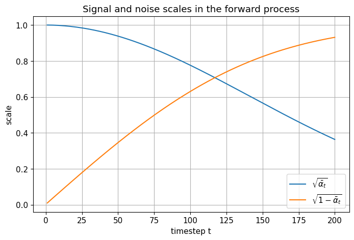
# Visualize alpha_bar_t and noise magnitude as a function of timestep

T = 200
betas, alphas, alpha_bars = make_linear_beta_schedule(T)
timesteps = np.arange(1, T + 1)

signal_scales = np.sqrt(alpha_bars)
noise_scales = np.sqrt(1.0 - alpha_bars)

plt.figure()
plt.plot(timesteps, signal_scales, label=r'$\sqrt{\bar{\alpha}_t}$')
plt.plot(timesteps, noise_scales, label=r'$\sqrt{1-\bar{\alpha}_t}$')
plt.xlabel("timestep t")
plt.ylabel("scale")
plt.title("Signal and noise scales in the forward process")
plt.legend()
plt.show()

DDIM Derivation

We now derive the DDIM update carefully.

Step 1: Start from the noisy-sample identity

At timestep \(t\),

\[ x_t = \sqrt{\bar\alpha_t}x_0 + \sqrt{1-\bar\alpha_t}\epsilon. \]

Solving for \(x_0\) gives

\[ x_0 = \frac{x_t - \sqrt{1-\bar\alpha_t}\epsilon}{\sqrt{\bar\alpha_t}}. \]

Replacing the unknown \(\epsilon\) by the network prediction yields

\[ \hat x_0 = \frac{x_t - \sqrt{1-\bar\alpha_t}\,\epsilon_\theta(x_t,t)}{\sqrt{\bar\alpha_t}}. \]

---

Step 2: Ask what a point at timestep \(t-1\) should look like

At timestep \(t-1\), the forward marginal would have the form

\[ x_{t-1} = \sqrt{\bar\alpha_{t-1}}x_0 + \sqrt{1-\bar\alpha_{t-1}}\epsilon'. \]

DDIM constructs a reverse step by using the estimated clean sample \(\hat x_0\) and decomposing the remaining noise budget into:

• a model-aligned direction term

• an optional fresh Gaussian term

So we write

\[ x_{t-1} = \sqrt{\bar\alpha_{t-1}}\,\hat x_0 + \sqrt{1-\bar\alpha_{t-1}-\sigma_t^2}\,\epsilon_\theta(x_t,t) + \sigma_t z, \qquad z \sim \mathcal N(0,I). \]

This is the generalized DDIM update.

---

Step 3: Why does the coefficient of \(\epsilon_\theta\) look like that?

At timestep \(t-1\), the total variance budget should be

\[ 1-\bar\alpha_{t-1}. \]

DDIM splits this budget into two parts:

\[ 1-\bar\alpha_{t-1} = \big(1-\bar\alpha_{t-1}-\sigma_t^2\big) + \sigma_t^2. \]

So:

• the direction term gets variance magnitude \(1-\bar\alpha_{t-1}-\sigma_t^2\)

• the fresh-noise term gets variance magnitude \(\sigma_t^2\)

This explains the structure

\[ \sqrt{1-\bar\alpha_{t-1}-\sigma_t^2}\,\epsilon_\theta(x_t,t). \]

---

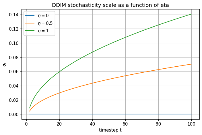
Step 4: Generalized DDIM variance scale

DDIM defines

\[ \sigma_t(\eta) = \eta \sqrt{ \frac{1-\bar\alpha_{t-1}}{1-\bar\alpha_t} \left( 1 - \frac{\bar\alpha_t}{\bar\alpha_{t-1}} \right) }. \]

This introduces the stochasticity parameter \(\eta\).

• \(\eta = 0\) gives deterministic DDIM

• \(\eta > 0\) gives stochastic DDIM

• \(\eta = 1\) matches DDPM posterior variance for adjacent steps

---

Step 5: Verify the DDPM consistency when \(\eta = 1\)

For adjacent steps,

\[ 1 - \frac{\bar\alpha_t}{\bar\alpha_{t-1}} = 1 - \alpha_t = \beta_t. \]

So

\[ \sigma_t^2 = \frac{1-\bar\alpha_{t-1}}{1-\bar\alpha_t}\beta_t = \tilde\beta_t. \]

Thus DDIM recovers the DDPM posterior variance when \(\eta = 1\).

---

Step 6: Deterministic DDIM

If \(\eta = 0\), then \(\sigma_t = 0\), and the update reduces to

\[ x_{t-1} = \sqrt{\bar\alpha_{t-1}}\,\hat x_0 + \sqrt{1-\bar\alpha_{t-1}}\,\epsilon_\theta(x_t,t). \]

No fresh noise is injected, so the trajectory is deterministic given the initial noise \(x_T\).

---

Step 7: Write DDIM fully in terms of \(x_t\) and \(\epsilon_\theta\)

Substitute

\[ \hat x_0 = \frac{x_t - \sqrt{1-\bar\alpha_t}\,\epsilon_\theta(x_t,t)}{\sqrt{\bar\alpha_t}} \]

into the DDIM update:

\[ x_{t-1} = \sqrt{\bar\alpha_{t-1}} \left( \frac{x_t - \sqrt{1-\bar\alpha_t}\,\epsilon_\theta(x_t,t)}{\sqrt{\bar\alpha_t}} \right) + \sqrt{1-\bar\alpha_{t-1}-\sigma_t^2}\,\epsilon_\theta(x_t,t) + \sigma_t z. \]

Expanding the first term gives

\[ x_{t-1} = \sqrt{\frac{\bar\alpha_{t-1}}{\bar\alpha_t}}\,x_t - \sqrt{\frac{\bar\alpha_{t-1}}{\bar\alpha_t}}\sqrt{1-\bar\alpha_t}\,\epsilon_\theta(x_t,t) + \sqrt{1-\bar\alpha_{t-1}-\sigma_t^2}\,\epsilon_\theta(x_t,t) + \sigma_t z. \]

Grouping the \(\epsilon_\theta\) terms gives

\[ x_{t-1} = \sqrt{\frac{\bar\alpha_{t-1}}{\bar\alpha_t}}\,x_t + \left( \sqrt{1-\bar\alpha_{t-1}-\sigma_t^2} - \sqrt{\frac{\bar\alpha_{t-1}}{\bar\alpha_t}}\sqrt{1-\bar\alpha_t} \right)\epsilon_\theta(x_t,t) + \sigma_t z. \]

This is an explicit DDIM update in terms of \(x_t\) and the predicted noise.

---

Step 8: Why DDIM differs from ancestral DDPM

DDPM ancestral sampling uses the posterior-inspired mean and fresh noise at every step.

DDIM instead explicitly reconstructs \(\hat x_0\) and then reprojects to a lower-noise point using a controlled mixture of:

• estimated clean content

• predicted direction

• optional randomness

This reparameterized viewpoint is what makes timestep skipping natural.

Show code cell source

Hide code cell source

def ddim_sigma(alpha_bar_t, alpha_bar_prev, eta):
    alpha_bar_t = float(alpha_bar_t)
    alpha_bar_prev = float(alpha_bar_prev)

    # If current time is effectively t=0, no reverse step should happen.
    if alpha_bar_t >= 1.0 - 1e-12:
        return 0.0

    inside = ((1.0 - alpha_bar_prev) / max(1.0 - alpha_bar_t, 1e-12)) * \
             max(1.0 - alpha_bar_t / max(alpha_bar_prev, 1e-12), 0.0)

    return float(eta) * np.sqrt(max(inside, 0.0))

def ddim_step_from_eps(x_t, eps_pred, alpha_bar_t, alpha_bar_prev, eta, rng=None):
    if rng is None:
        rng = np.random.default_rng()

    alpha_bar_t = float(alpha_bar_t)
    alpha_bar_prev = float(alpha_bar_prev)

    x0_hat = x0_from_eps(x_t, eps_pred, alpha_bar_t)
    sigma_t = ddim_sigma(alpha_bar_t, alpha_bar_prev, eta)

    dir_coeff_sq = max(1.0 - alpha_bar_prev - sigma_t**2, 0.0)
    dir_coeff = np.sqrt(dir_coeff_sq)

    z = rng.normal(size=np.shape(x_t))
    x_prev = np.sqrt(max(alpha_bar_prev, 0.0)) * x0_hat + dir_coeff * eps_pred + sigma_t * z
    return x_prev, x0_hat, sigma_t

def ddim_step_from_x0(x_t, x0_hat, alpha_bar_t, alpha_bar_prev, eta, rng=None):
    eps_pred = eps_from_x0(x_t, x0_hat, alpha_bar_t)
    return ddim_step_from_eps(x_t, eps_pred, alpha_bar_t, alpha_bar_prev, eta, rng=rng)

def ddim_step_general(x_t, eps_pred, alpha_bar_t, alpha_bar_s, eta, rng=None):
    """
    General DDIM step from current timestep t to target timestep s, where s < t.
    alpha_bar_t = current cumulative alpha
    alpha_bar_s = target cumulative alpha
    """
    if rng is None:
        rng = np.random.default_rng()

    alpha_bar_t = float(alpha_bar_t)
    alpha_bar_s = float(alpha_bar_s)

    # Reverse stepping should never start from t = 0
    if alpha_bar_t >= 1.0 - 1e-12:
        raise ValueError("ddim_step_general was called with current timestep t=0. Reverse stepping should stop at x_0.")

    x0_hat = x0_from_eps(x_t, eps_pred, alpha_bar_t)

    inside = ((1.0 - alpha_bar_s) / max(1.0 - alpha_bar_t, 1e-12)) * \
             max(1.0 - alpha_bar_t / max(alpha_bar_s, 1e-12), 0.0)

    sigma_ts = float(eta) * np.sqrt(max(inside, 0.0))

    dir_coeff_sq = max(1.0 - alpha_bar_s - sigma_ts**2, 0.0)
    dir_coeff = np.sqrt(dir_coeff_sq)

    z = rng.normal(size=np.shape(x_t))
    x_s = np.sqrt(max(alpha_bar_s, 0.0)) * x0_hat + dir_coeff * eps_pred + sigma_ts * z
    return x_s, x0_hat, sigma_ts

# Compare the DDIM sigma_t as eta varies

T = 100
betas, alphas, alpha_bars = make_linear_beta_schedule(T)

ts = np.arange(2, T + 1)
sigma_eta0 = []
sigma_eta05 = []
sigma_eta1 = []

for t in ts:
    alpha_bar_t = get_alpha_bar(alpha_bars, t)
    alpha_bar_prev = get_alpha_bar(alpha_bars, t - 1)
    sigma_eta0.append(ddim_sigma(alpha_bar_t, alpha_bar_prev, eta=0.0))
    sigma_eta05.append(ddim_sigma(alpha_bar_t, alpha_bar_prev, eta=0.5))
    sigma_eta1.append(ddim_sigma(alpha_bar_t, alpha_bar_prev, eta=1.0))

plt.figure()
plt.plot(ts, sigma_eta0, label=r'$\eta=0$')
plt.plot(ts, sigma_eta05, label=r'$\eta=0.5$')
plt.plot(ts, sigma_eta1, label=r'$\eta=1$')
plt.xlabel("timestep t")
plt.ylabel(r'$\sigma_t$')
plt.title("DDIM stochasticity scale as a function of eta")
plt.legend()
plt.show()

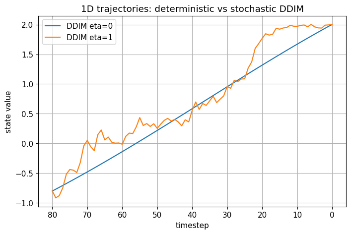
Deterministic vs Stochastic DDIM

The DDIM update is

\[ x_{t-1} = \sqrt{\bar\alpha_{t-1}}\,\hat x_0 + \sqrt{1-\bar\alpha_{t-1}-\sigma_t^2}\,\epsilon_\theta(x_t,t) + \sigma_t z. \]

The only source of fresh randomness is the final term \(\sigma_t z\).

---

Deterministic DDIM

When \(\eta = 0\),

\[ \sigma_t = 0, \]

so

\[ x_{t-1} = \sqrt{\bar\alpha_{t-1}}\,\hat x_0 + \sqrt{1-\bar\alpha_{t-1}}\,\epsilon_\theta(x_t,t). \]

This means:

• no fresh noise is injected

• the trajectory is fully determined by the starting point \(x_T\)

• trajectories are often smoother

• interpolation and inversion become more natural

---

Stochastic DDIM

When \(\eta > 0\),

\[ x_{t-1} = \sqrt{\bar\alpha_{t-1}}\,\hat x_0 + \sqrt{1-\bar\alpha_{t-1}-\sigma_t^2}\,\epsilon_\theta(x_t,t) + \sigma_t z. \]

Now the reverse process has two distinct sources of uncertainty:

1. the initial random sample \(x_T\)

2. fresh per-step noise \(\sigma_t z\)

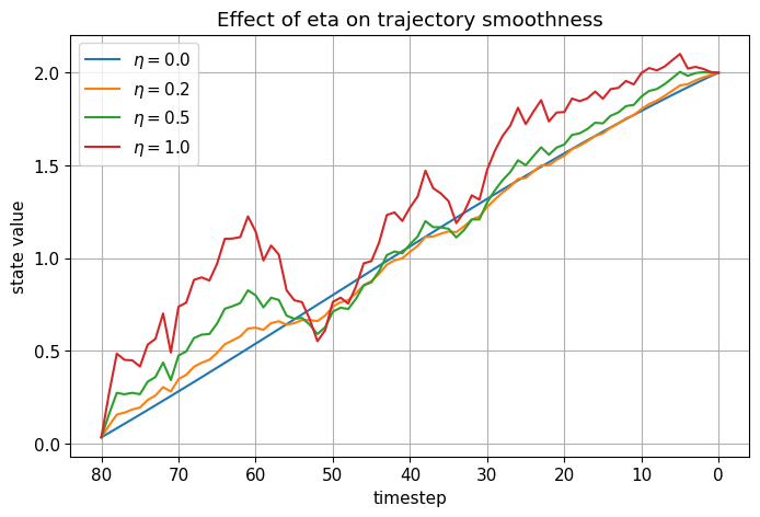
As \(\eta\) increases, trajectories become less deterministic and more diverse.

---

Trajectory smoothness intuition

In deterministic DDIM, the sequence evolves by repeatedly:

1. estimating the same underlying clean content

2. re-expressing that content at progressively lower noise levels

So the latent path is often smoother than in DDPM ancestral sampling, which injects fresh perturbations at every step.

# 1D pedagogical trajectory comparison: deterministic vs stochastic DDIM

T = 80
betas, alphas, alpha_bars = make_linear_beta_schedule(T)
rng = np.random.default_rng(7)

def true_eps_model(x_t, t, x0_true, alpha_bars):
    alpha_bar_t = get_alpha_bar(alpha_bars, t)
    return eps_from_x0(x_t, np.array([x0_true]), alpha_bar_t)

def simulate_ddim_trajectory(x0_true=2.0, xT=None, eta=0.0, T=80, seed=0):
    betas, alphas, alpha_bars = make_linear_beta_schedule(T)
    rng = np.random.default_rng(seed)
    if xT is None:
        x_t = rng.normal(size=(1,))
    else:
        x_t = np.array([xT], dtype=np.float64)

    traj = [(T, x_t.item())]
    for t in range(T, 0, -1):
        alpha_bar_t = get_alpha_bar(alpha_bars, t)
        alpha_bar_prev = get_alpha_bar(alpha_bars, t - 1)
        eps_pred = true_eps_model(x_t, t, x0_true, alpha_bars)
        x_t, _, _ = ddim_step_from_eps(x_t, eps_pred, alpha_bar_t, alpha_bar_prev, eta=eta, rng=rng)
        traj.append((t - 1, x_t.item()))
    return traj

traj_det = simulate_ddim_trajectory(eta=0.0, seed=5)
traj_sto = simulate_ddim_trajectory(eta=1.0, seed=5)

plt.figure()
plt.plot([t for t, x in traj_det], [x for t, x in traj_det], label="DDIM eta=0")
plt.plot([t for t, x in traj_sto], [x for t, x in traj_sto], label="DDIM eta=1")
plt.gca().invert_xaxis()
plt.xlabel("timestep")
plt.ylabel("state value")
plt.title("1D trajectories: deterministic vs stochastic DDIM")
plt.legend()
plt.show()

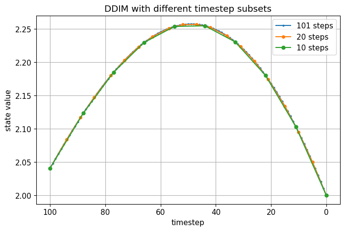
Timestep Sub-Sampling

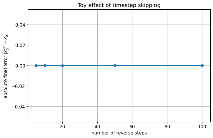
One of the main practical advantages of DDIM is that it supports reduced-step sampling naturally.

Instead of using every timestep

\[ T, T-1, \dots, 1, 0, \]

we choose a subsequence

\[ \tau_0 = T > \tau_1 > \cdots > \tau_S = 0. \]

At each step, we move directly from \(x_{\tau_i}\) to \(x_{\tau_{i+1}}\).

---

General DDIM update for skipped steps

Let \(t = \tau_i\) and \(s = \tau_{i+1}\) with \(s < t\). Then the generalized DDIM update is

\[ x_s = \sqrt{\bar\alpha_s}\,\hat x_0 + \sqrt{1-\bar\alpha_s-\sigma_{t\to s}^2}\,\epsilon_\theta(x_t,t) + \sigma_{t\to s} z, \]

where

\[ \sigma_{t\to s}(\eta) = \eta \sqrt{ \frac{1-\bar\alpha_s}{1-\bar\alpha_t} \left( 1-\frac{\bar\alpha_t}{\bar\alpha_s} \right) }. \]

This is the skipped-step analogue of the adjacent-step DDIM update.

---

Why skipping works

Once we have \(\hat x_0\), we can synthesize a point at another noise level because the forward marginal form at timestep \(s\) is

\[ x_s = \sqrt{\bar\alpha_s}x_0 + \sqrt{1-\bar\alpha_s}\epsilon. \]

DDIM uses the estimated clean sample and the model-predicted direction to jump directly between noise levels.

This is why DDIM is much more naturally compatible with accelerated sampling than ancestral DDPM.

---

What changes mathematically from DDPM?

In ancestral DDPM, the sampler is tied closely to adjacent-step posterior transitions.

In DDIM, the update is reparameterized in terms of:

• \(\hat x_0\)

• the target cumulative noise level \(\bar\alpha_s\)

• a chosen stochasticity level \(\eta\)

This makes step skipping a first-class part of the sampler.

Show code cell source

Hide code cell source

def make_timestep_subsequence(T, num_steps):
    # Descending sequence from T to 0
    seq = np.linspace(T, 0, num_steps, dtype=int)
    seq = np.unique(seq)[::-1]

    if seq[0] != T:
        seq = np.insert(seq, 0, T)
    if seq[-1] != 0:
        seq = np.append(seq, 0)

    return seq

def simulate_ddim_subsampled(x0_true=2.0, T=100, num_steps=20, eta=0.0, seed=0):
    betas, alphas, alpha_bars = make_linear_beta_schedule(T)
    rng = np.random.default_rng(seed)
    x_t = rng.normal(size=(1,))
    seq = make_timestep_subsequence(T, num_steps)

    traj = [(int(seq[0]), x_t.item())]

    for i in range(len(seq) - 1):
        t = int(seq[i])
        s = int(seq[i + 1])

        # Stop once we are already at x_0
        if t == 0:
            break

        alpha_bar_t = get_alpha_bar(alpha_bars, t)
        alpha_bar_s = get_alpha_bar(alpha_bars, s)

        eps_pred = true_eps_model(x_t, t, x0_true, alpha_bars)
        x_t, _, _ = ddim_step_general(x_t, eps_pred, alpha_bar_t, alpha_bar_s, eta=eta, rng=rng)
        traj.append((s, x_t.item()))

    return seq, traj

# Compare dense vs sparse DDIM timestep sequences

seq1, traj1 = simulate_ddim_subsampled(T=100, num_steps=101, eta=0.0, seed=3)
seq2, traj2 = simulate_ddim_subsampled(T=100, num_steps=20, eta=0.0, seed=3)
seq3, traj3 = simulate_ddim_subsampled(T=100, num_steps=10, eta=0.0, seed=3)

plt.figure()
plt.plot([t for t, x in traj1], [x for t, x in traj1], marker='o', ms=2, label='101 steps')
plt.plot([t for t, x in traj2], [x for t, x in traj2], marker='o', ms=4, label='20 steps')
plt.plot([t for t, x in traj3], [x for t, x in traj3], marker='o', ms=5, label='10 steps')
plt.gca().invert_xaxis()
plt.xlabel("timestep")
plt.ylabel("state value")
plt.title("DDIM with different timestep subsets")
plt.legend()
plt.show()

How \(\hat x_0\) and \(\epsilon_\theta\) Determine the Update

A very important practical point is that the reverse step can be written in multiple equivalent parameterizations.

From \(\epsilon_\theta\) to \(\hat x_0\)

If the model predicts noise, then

\[ \hat x_0 = \frac{x_t - \sqrt{1-\bar\alpha_t}\,\epsilon_\theta(x_t,t)}{\sqrt{\bar\alpha_t}}. \]

Then DDIM uses

\[ x_{t-1} = \sqrt{\bar\alpha_{t-1}}\,\hat x_0 + \sqrt{1-\bar\alpha_{t-1}-\sigma_t^2}\,\epsilon_\theta(x_t,t) + \sigma_t z. \]

---

From \(\hat x_0\) to \(\epsilon_\theta\)

If the model instead predicts \(\hat x_0\) directly, then the implied noise is

\[ \hat\epsilon = \frac{x_t - \sqrt{\bar\alpha_t}\,\hat x_0}{\sqrt{1-\bar\alpha_t}}. \]

Then the same DDIM formula applies after substitution.

---

Why this matters

This shows that DDIM is fundamentally a sampling framework, not a commitment to only one network output parameterization.

As long as we can consistently recover:

• \(\hat x_0\)

• and/or the denoising direction \(\hat\epsilon\)

we can execute the DDIM update.

# Demonstrate consistency between x0-prediction and epsilon-prediction for one DDIM step

T = 100
betas, alphas, alpha_bars = make_linear_beta_schedule(T)

t = 70
alpha_bar_t = get_alpha_bar(alpha_bars, t)
alpha_bar_prev = get_alpha_bar(alpha_bars, t - 1)

x_t = np.array([1.2])
eps_pred = np.array([-0.35])

x0_hat = x0_from_eps(x_t, eps_pred, alpha_bar_t)
eps_recovered = eps_from_x0(x_t, x0_hat, alpha_bar_t)

rng = np.random.default_rng(0)
x_prev_eps, _, sigma_eps = ddim_step_from_eps(x_t, eps_pred, alpha_bar_t, alpha_bar_prev, eta=0.0, rng=rng)

rng = np.random.default_rng(0)
x_prev_x0, _, sigma_x0 = ddim_step_from_x0(x_t, x0_hat, alpha_bar_t, alpha_bar_prev, eta=0.0, rng=rng)

print("x0_hat =", x0_hat)
print("eps recovered from x0_hat =", eps_recovered)
print("x_prev from eps =", x_prev_eps)
print("x_prev from x0 =", x_prev_x0)
print("difference =", np.abs(x_prev_eps - x_prev_x0))

x0_hat = [1.81682758]
eps recovered from x0_hat = [-0.35]
x_prev from eps = [1.21244742]
x_prev from x0 = [1.21244742]
difference = [0.]

Classifier Guidance

We now discuss conditional guidance after DDIM itself is fully established.

Score decomposition

For class-conditional generation with label \(y\), Bayes’ rule gives

\[ \log p_t(x_t \mid y) = \log p_t(x_t) + \log p_t(y \mid x_t) - \log p_t(y). \]

Differentiate with respect to \(x_t\):

\[ \nabla_{x_t}\log p_t(x_t \mid y) = \nabla_{x_t}\log p_t(x_t) + \nabla_{x_t}\log p_t(y \mid x_t). \]

So the conditional score equals the unconditional score plus a classifier gradient term.

---

Guided score

If \(s_\theta(x_t,t)\) denotes the unconditional reverse score, classifier guidance defines

\[ s_{\text{guided}}(x_t,t,y) = s_\theta(x_t,t) + w\,\nabla_{x_t}\log p_\phi(y\mid x_t,t), \]

where:

• \(p_\phi(y\mid x_t,t)\) is a classifier trained on noisy samples

• \(w\) is the guidance scale

---

Convert to \(\epsilon\)-prediction form

For variance-preserving diffusion, the score and noise prediction are related by

\[ s_\theta(x_t,t) \approx -\frac{1}{\sqrt{1-\bar\alpha_t}}\epsilon_\theta(x_t,t). \]

Therefore the guided \(\epsilon\) prediction becomes

\[ \epsilon_{\text{guided}} = \epsilon_\theta - w\sqrt{1-\bar\alpha_t}\,\nabla_{x_t}\log p_\phi(y\mid x_t,t). \]

This is the quantity used inside DDPM or DDIM sampling.

---

Connection to DDIM

Once we have \(\epsilon_{\text{guided}}\), we simply replace \(\epsilon_\theta\) by \(\epsilon_{\text{guided}}\) in the DDIM step:

\[ \hat x_0 = \frac{x_t - \sqrt{1-\bar\alpha_t}\,\epsilon_{\text{guided}}}{\sqrt{\bar\alpha_t}}, \]

and

\[ x_{t-1} = \sqrt{\bar\alpha_{t-1}}\,\hat x_0 + \sqrt{1-\bar\alpha_{t-1}-\sigma_t^2}\,\epsilon_{\text{guided}} + \sigma_t z. \]

So guidance is orthogonal to the DDPM-vs-DDIM distinction: it modifies the denoising direction used by either sampler.

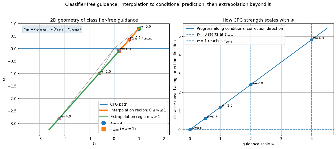
Classifier-Free Guidance

Classifier-free guidance avoids training a separate classifier.

Basic idea

During training, the diffusion model is trained both:

• conditionally on \(y\)

• unconditionally, by dropping the condition with some probability

So the same model learns:

• \(\epsilon_\theta(x_t,t,y)\)

• \(\epsilon_\theta(x_t,t,\varnothing)\)

---

CFG formula

The standard classifier-free guidance combination is

\[ \epsilon_{\text{cfg}}(x_t,t,y) = \epsilon_\theta(x_t,t,\varnothing) + w\Big( \epsilon_\theta(x_t,t,y) - \epsilon_\theta(x_t,t,\varnothing) \Big). \]

Equivalent form:

\[ \epsilon_{\text{cfg}} = (1-w)\epsilon_\theta(x_t,t,\varnothing) + w\,\epsilon_\theta(x_t,t,y). \]

---

Interpretation

• \(\epsilon_\theta(x_t,t,\varnothing)\) is the unconditional denoising direction

• \(\epsilon_\theta(x_t,t,y)\) is the conditional denoising direction

• the difference estimates the conditional correction

• \(w\) amplifies or attenuates that correction

Special cases:

• \(w = 0\): unconditional sampling

• \(w = 1\): ordinary conditional sampling

• \(w > 1\): extrapolated guidance, often stronger prompt/class alignment

---

Tradeoff between fidelity and diversity

As guidance scale \(w\) increases:

• condition alignment usually improves

• diversity often decreases

• oversharpening or artifacts may appear at very high scales

This tradeoff exists for both DDPM and DDIM samplers.

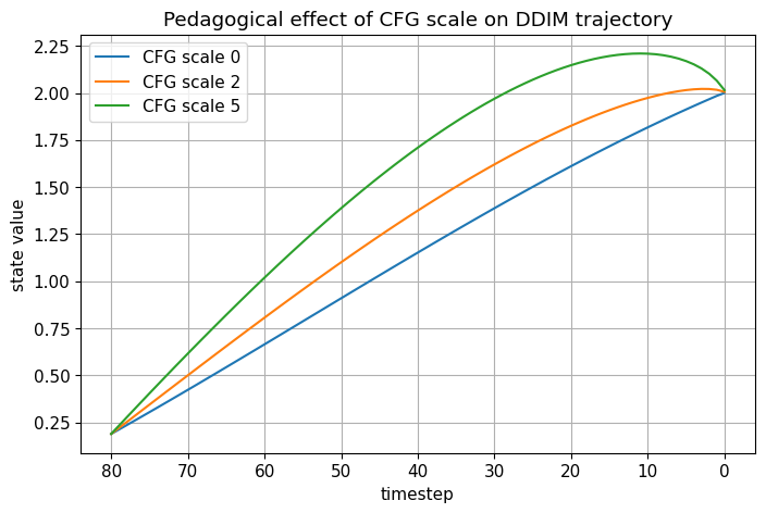
In deterministic or low-noise DDIM, strong guidance can make trajectories especially rigid.

Algorithm: DDIM Sampling

Below is the algorithmic structure for DDIM sampling.

Inputs

• trained denoiser \(\epsilon_\theta(x_t,t)\)

• noise schedule \(\{\alpha_t\}_{t=1}^T\)

• cumulative schedule \(\bar\alpha_t = \prod_{s=1}^t \alpha_s\)

• timestep subsequence \(\tau_0 = T > \tau_1 > \cdots > \tau_S = 0\)

• stochasticity parameter \(\eta\)

• initial noise \(x_{\tau_0} \sim \mathcal N(0,I)\)

DDIM sampling algorithm

For \(i = 0, 1, \dots, S-1\):

1. set \(t = \tau_i\) and \(s = \tau_{i+1}\)

2. predict noise:

   \[ \epsilon_t = \epsilon_\theta(x_t, t) \]

3. reconstruct clean sample:

   \[ \hat x_0 = \frac{x_t - \sqrt{1-\bar\alpha_t}\,\epsilon_t}{\sqrt{\bar\alpha_t}} \]

4. compute stochasticity scale:

   \[ \sigma_{t\to s} = \eta \sqrt{ \frac{1-\bar\alpha_s}{1-\bar\alpha_t} \left( 1-\frac{\bar\alpha_t}{\bar\alpha_s} \right) } \]

5. sample \(z \sim \mathcal N(0,I)\) if \(\eta > 0\)

6. update:

   \[ x_s = \sqrt{\bar\alpha_s}\,\hat x_0 + \sqrt{1-\bar\alpha_s-\sigma_{t\to s}^2}\,\epsilon_t + \sigma_{t\to s} z \]

Output \(x_0\).

---

Important interpretation

This algorithm differs from ancestral DDPM in two ways:

1. it is written in reparameterized form using \(\hat x_0\)

2. it naturally allows sparse timestep subsets

Algorithm: DDIM Sampling with Classifier-Free Guidance

Now we include classifier-free guidance inside DDIM.

Inputs

• conditional denoiser outputs:

  • \(\epsilon_\theta(x_t,t,\varnothing)\)

  • \(\epsilon_\theta(x_t,t,y)\)

• guidance scale \(w\)

• all DDIM inputs from the previous section

CFG-DDIM algorithm

For each reverse step from \(t\) to \(s\):

1. compute unconditional prediction:

   \[ \epsilon_u = \epsilon_\theta(x_t,t,\varnothing) \]

2. compute conditional prediction:

   \[ \epsilon_c = \epsilon_\theta(x_t,t,y) \]

3. combine using classifier-free guidance:

   \[ \epsilon_{\text{cfg}} = \epsilon_u + w(\epsilon_c - \epsilon_u) \]

4. reconstruct clean sample:

   \[ \hat x_0 = \frac{x_t - \sqrt{1-\bar\alpha_t}\,\epsilon_{\text{cfg}}}{\sqrt{\bar\alpha_t}} \]

5. compute \(\sigma_{t\to s}(\eta)\)

6. update:

   \[ x_s = \sqrt{\bar\alpha_s}\,\hat x_0 + \sqrt{1-\bar\alpha_s-\sigma_{t\to s}^2}\,\epsilon_{\text{cfg}} + \sigma_{t\to s} z \]

Output the final \(x_0\).

---

Interpretation

CFG changes the denoising direction before the sampler update is applied.
The DDIM structure remains the same; only the effective \(\epsilon\) prediction changes.

# Simplified pedagogical DDIM + CFG trajectory demo in 1D

T = 80
betas, alphas, alpha_bars = make_linear_beta_schedule(T)

def simulate_cfg_ddim_trajectory(x0_true=2.0, cond_bias=-0.3, guidance_scale=0.0, eta=0.0, seed=0):
    rng = np.random.default_rng(seed)
    x_t = rng.normal(size=(1,))
    traj = [(T, x_t.item())]

    for t in range(T, 0, -1):
        alpha_bar_t = get_alpha_bar(alpha_bars, t)
        alpha_bar_prev = get_alpha_bar(alpha_bars, t - 1)

        # unconditional "teacher"
        eps_uncond = eps_from_x0(x_t, np.array([x0_true]), alpha_bar_t)

        # conditional branch = perturbed direction in a pedagogical way
        eps_cond = eps_uncond + cond_bias

        eps_guided = cfg_eps(eps_uncond, eps_cond, guidance_scale)
        x_t, _, _ = ddim_step_from_eps(x_t, eps_guided, alpha_bar_t, alpha_bar_prev, eta=eta, rng=rng)
        traj.append((t - 1, x_t.item()))
    return traj

traj_w0 = simulate_cfg_ddim_trajectory(guidance_scale=0.0, eta=0.0, seed=2)
traj_w2 = simulate_cfg_ddim_trajectory(guidance_scale=2.0, eta=0.0, seed=2)
traj_w5 = simulate_cfg_ddim_trajectory(guidance_scale=5.0, eta=0.0, seed=2)

plt.figure()
plt.plot([t for t, x in traj_w0], [x for t, x in traj_w0], label='CFG scale 0')
plt.plot([t for t, x in traj_w2], [x for t, x in traj_w2], label='CFG scale 2')
plt.plot([t for t, x in traj_w5], [x for t, x in traj_w5], label='CFG scale 5')
plt.gca().invert_xaxis()
plt.xlabel("timestep")
plt.ylabel("state value")
plt.title("Pedagogical effect of CFG scale on DDIM trajectory")
plt.legend()
plt.show()

Compact Comparison: DDPM vs DDIM vs DDIM + CFG

This section summarizes the practical differences.

DDPM ancestral sampling

Update:

\[ x_{t-1} = \mu_\theta(x_t,t) + \sigma_t z \]

Characteristics:

• stochastic at every step

• closely tied to the posterior structure

• usually many steps

• good diversity due to repeated noise injection

---

DDIM

Update:

\[ x_{t-1} = \sqrt{\bar\alpha_{t-1}}\,\hat x_0 + \sqrt{1-\bar\alpha_{t-1}-\sigma_t^2}\,\epsilon_\theta + \sigma_t z \]

Characteristics:

• can be deterministic when \(\eta=0\)

• naturally supports timestep skipping

• often much faster

• often smoother latent trajectories

• diversity may reduce when \(\eta\) is very small

---

DDIM + CFG

Update uses guided noise prediction

\[ \epsilon_{\text{cfg}} = \epsilon_\theta(x_t,t,\varnothing) + w\big(\epsilon_\theta(x_t,t,y)-\epsilon_\theta(x_t,t,\varnothing)\big) \]

and then the usual DDIM formula.

Characteristics:

• inherits DDIM speed and controllability

• improves condition fidelity

• may reduce diversity as guidance scale increases

• strong guidance can produce rigid trajectories or artifacts

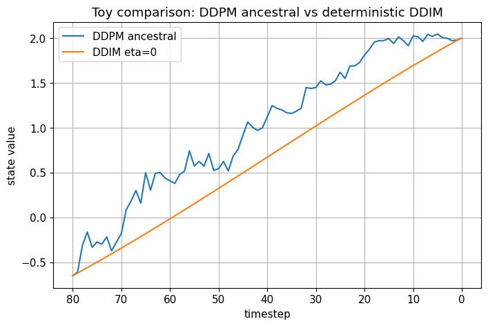
# Compare DDPM-style stochastic update and DDIM deterministic update in a 1D toy setting

T = 80
betas, alphas, alpha_bars = make_linear_beta_schedule(T)

def simulate_ddpm_ancestral_trajectory(x0_true=2.0, T=80, seed=0):
    rng = np.random.default_rng(seed)
    x_t = rng.normal(size=(1,))
    traj = [(T, x_t.item())]
    for t in range(T, 0, -1):
        beta_t = betas[t - 1]
        alpha_t = alphas[t - 1]
        alpha_bar_t = get_alpha_bar(alpha_bars, t)
        alpha_bar_prev = get_alpha_bar(alpha_bars, t - 1)
        eps_pred = eps_from_x0(x_t, np.array([x0_true]), alpha_bar_t)
        mu = ddpm_mean_from_eps(x_t, eps_pred, alpha_t, alpha_bar_t)
        sigma = np.sqrt(posterior_variance(beta_t, alpha_bar_t, alpha_bar_prev))
        x_t = mu + sigma * rng.normal(size=(1,))
        traj.append((t - 1, x_t.item()))
    return traj

traj_ddpm = simulate_ddpm_ancestral_trajectory(seed=4)
traj_ddim = simulate_ddim_trajectory(eta=0.0, seed=4)

plt.figure()
plt.plot([t for t, x in traj_ddpm], [x for t, x in traj_ddpm], label='DDPM ancestral')
plt.plot([t for t, x in traj_ddim], [x for t, x in traj_ddim], label='DDIM eta=0')
plt.gca().invert_xaxis()
plt.xlabel("timestep")
plt.ylabel("state value")
plt.title("Toy comparison: DDPM ancestral vs deterministic DDIM")
plt.legend()
plt.show()

Implementation Notes

This section summarizes the key implementation choices.

1. The model can predict different quantities

The sampler may be implemented using:

• \(\epsilon\)-prediction

• \(x_0\)-prediction

• \(v\)-prediction

But the DDIM step is easiest to think about in terms of \(\hat x_0\) and \(\hat\epsilon\).

---

2. Use a helper to reconstruct \(\hat x_0\)

For \(\epsilon\)-prediction:

\[ \hat x_0 = \frac{x_t - \sqrt{1-\bar\alpha_t}\,\epsilon_\theta(x_t,t)}{\sqrt{\bar\alpha_t}}. \]

This helper is central and should be implemented carefully.

---

3. Timestep skipping requires a chosen sequence

Instead of all timesteps, select a sequence such as:

• uniform in index

• quadratic spacing

• custom hand-designed schedules

The DDIM formulas use the corresponding \(\bar\alpha_t\) values directly.

---

4. Deterministic DDIM is often used for inversion/editing

Because the mapping is deterministic given the initial noise, DDIM is often used when we want more stable trajectories, interpolation, or inversion-style reasoning.

---

5. Guidance is inserted before the sampler update

For classifier-free guidance:

1. get unconditional prediction

2. get conditional prediction

3. combine them to get \(\epsilon_{\text{cfg}}\)

4. use \(\epsilon_{\text{cfg}}\) inside the DDIM update

So guidance modifies the denoiser output, not the structural form of the DDIM formula.

---

6. Numerical stability

In practice, implementations often:

• clip or threshold \(\hat x_0\)

• ensure square-root arguments are nonnegative

• use precomputed tensors for \(\alpha_t\) and \(\bar\alpha_t\)

• carefully handle timestep indexing conventions

# Show how eta affects trajectory smoothness by plotting several trajectories from the same start

etas = [0.0, 0.2, 0.5, 1.0]
plt.figure()

for eta in etas:
    traj = simulate_ddim_trajectory(eta=eta, seed=11)
    plt.plot([t for t, x in traj], [x for t, x in traj], label=fr'$\eta={eta}$')

plt.gca().invert_xaxis()
plt.xlabel("timestep")
plt.ylabel("state value")
plt.title("Effect of eta on trajectory smoothness")
plt.legend()
plt.show()

# Visualize the effect of timestep skipping on final error in a toy setting

T = 100
x0_true = 2.0
step_counts = [100, 50, 20, 10, 5]
final_errors = []

for num_steps in step_counts:
    _, traj = simulate_ddim_subsampled(x0_true=x0_true, T=T, num_steps=num_steps, eta=0.0, seed=13)
    x0_est = traj[-1][1]
    final_errors.append(abs(x0_est - x0_true))

plt.figure()
plt.plot(step_counts, final_errors, marker='o')
plt.xlabel("number of reverse steps")
plt.ylabel(r"absolute final error $|x_0^{\mathrm{est}} - x_0|$")
plt.title("Toy effect of timestep skipping")
plt.show()

Common Confusions

1. Is DDIM a new training objective?

Not necessarily. The key practical point is that DDIM reuses the same denoiser trained under the DDPM-style objective. What changes is the sampler.

---

2. Is DDIM just DDPM with no noise?

That is only partly true. Deterministic DDIM is the \(\eta=0\) limit, but DDIM is more generally a family of reparameterized samplers that also supports arbitrary timestep skipping.

---

3. Why does deterministic DDIM still generate diverse samples?

Because the initial state \(x_T\) is still sampled from a random Gaussian. The reverse path is deterministic conditioned on this initial point, but the overall generative model remains random through its starting noise.

---

4. Why is DDIM often said to be non-Markovian?

The main idea is that DDIM corresponds to a broader process family that preserves the same marginals \(q(x_t\mid x_0)\) while not being tied to the original DDPM ancestral Markov chain interpretation.

---

5. Why do smoother trajectories appear in DDIM?

Because deterministic or low-noise DDIM does not inject fresh Gaussian perturbations at every step. Instead, it repeatedly projects the estimated clean content to lower-noise levels.

---

6. Is guidance specific to DDIM?

No. Guidance modifies the denoising direction and can be used with DDPM, DDIM, and many other diffusion samplers.

---

7. Why can very large guidance scale hurt samples?

Because it over-amplifies the conditional correction. This usually improves fidelity to the condition but can reduce diversity and produce unnatural or oversharpened outputs.

Summary

We can now summarize the full notebook in a compact way.

Core DDIM idea

Given a noisy point \(x_t\), use the denoiser to reconstruct

\[ \hat x_0 = \frac{x_t - \sqrt{1-\bar\alpha_t}\,\epsilon_\theta(x_t,t)}{\sqrt{\bar\alpha_t}}. \]

Then move to a lower noise level using

\[ x_{t-1} = \sqrt{\bar\alpha_{t-1}}\,\hat x_0 + \sqrt{1-\bar\alpha_{t-1}-\sigma_t^2}\,\epsilon_\theta(x_t,t) + \sigma_t z. \]

---

What DDIM changes relative to DDPM

DDPM:

• ancestral posterior-style sampling

• fresh noise every step

• often many reverse steps

DDIM:

• reparameterized update via \(\hat x_0\)

• optional stochasticity controlled by \(\eta\)

• natural timestep skipping

• deterministic generation when \(\eta = 0\)

---

Why DDIM is useful

DDIM is important because it offers:

• faster sampling

• smoother trajectories

• deterministic paths for inversion/interpolation

• compatibility with guidance methods

---

Final conceptual takeaway

DDIM should be understood as a sampler family built on top of the DDPM denoiser.
The model training can stay the same, while the reverse-time generation path becomes more flexible, faster, and in special cases deterministic.

Once Loop Reflect

Show code cell source

Hide code cell source

import numpy as np
import matplotlib.pyplot as plt

# ============================================================
# 1. Dataset
# ============================================================
def make_pinwheel(
    n_samples=4000,
    radial_std=0.18,
    tangential_std=0.06,
    num_classes=3,
    rate=0.18,
    scale=2.0,
    seed=7,
):
    rng = np.random.default_rng(seed)

    counts = np.full(num_classes, n_samples // num_classes, dtype=int)
    counts[: n_samples % num_classes] += 1

    labels = np.concatenate([
        np.full(c, k, dtype=int) for k, c in enumerate(counts)
    ])

    r = rng.normal(loc=1.0, scale=radial_std, size=n_samples)
    t = rng.normal(loc=0.0, scale=tangential_std, size=n_samples)

    base = 2.0 * np.pi * labels / num_classes
    angles = base + rate * np.exp(r) + t

    x = np.stack([r * np.cos(angles), r * np.sin(angles)], axis=1)
    x *= scale

    perm = rng.permutation(n_samples)
    return x[perm], labels[perm]


# ============================================================
# 2. Normalization helpers
# ============================================================
def normalize_data(x):
    mean = x.mean(axis=0, keepdims=True)
    std = x.std(axis=0, keepdims=True) + 1e-8
    x_norm = (x - mean) / std
    stats = {"mean": mean, "std": std}
    return x_norm, stats

def denormalize_data(x_norm, stats):
    return x_norm * stats["std"] + stats["mean"]


# ============================================================
# 3. Diffusion schedule helpers
# ============================================================
def make_linear_beta_schedule(T, beta_start=1e-4, beta_end=2e-2):
    betas = np.linspace(beta_start, beta_end, T, dtype=np.float64)
    alphas = 1.0 - betas
    alpha_bars = np.cumprod(alphas)
    return betas, alphas, alpha_bars

def get_alpha_bar(alpha_bars, t):
    if t == 0:
        return 1.0
    return float(alpha_bars[t - 1])

def sample_q_xt_given_x0(x0, t_indices, alpha_bars, rng):
    alpha_bar_t = alpha_bars[t_indices - 1][:, None]
    eps = rng.normal(size=x0.shape)
    x_t = np.sqrt(alpha_bar_t) * x0 + np.sqrt(1.0 - alpha_bar_t) * eps
    return x_t, eps

def x0_from_eps(x_t, eps_pred, alpha_bar_t, eps=1e-12):
    return (x_t - np.sqrt(max(1.0 - alpha_bar_t, 0.0)) * eps_pred) / np.sqrt(max(alpha_bar_t, eps))

def ddim_sigma(alpha_bar_t, alpha_bar_s, eta, eps=1e-12):
    if alpha_bar_t >= 1.0 - eps:
        return 0.0
    inside = ((1.0 - alpha_bar_s) / max(1.0 - alpha_bar_t, eps)) * \
             max(1.0 - alpha_bar_t / max(alpha_bar_s, eps), 0.0)
    return float(eta) * np.sqrt(max(inside, 0.0))

def ddim_step_general(x_t, eps_pred, alpha_bar_t, alpha_bar_s, eta, rng):
    x0_hat = x0_from_eps(x_t, eps_pred, alpha_bar_t)
    sigma_ts = ddim_sigma(alpha_bar_t, alpha_bar_s, eta)
    dir_coeff = np.sqrt(max(1.0 - alpha_bar_s - sigma_ts**2, 0.0))
    z = rng.normal(size=x_t.shape)
    x_s = np.sqrt(max(alpha_bar_s, 0.0)) * x0_hat + dir_coeff * eps_pred + sigma_ts * z
    return x_s, x0_hat, sigma_ts

def make_timestep_subsequence(T, num_steps):
    seq = np.linspace(T, 0, num_steps, dtype=int)
    seq = np.unique(seq)[::-1]
    if seq[0] != T:
        seq = np.insert(seq, 0, T)
    if seq[-1] != 0:
        seq = np.append(seq, 0)
    return seq


# ============================================================
# 4. Sinusoidal timestep embedding
# ============================================================
def timestep_embedding(t_indices, dim, T):
    t = np.asarray(t_indices, dtype=np.float64)[:, None] / float(T)
    half = dim // 2
    freqs = np.exp(-np.log(10000.0) * np.arange(half) / max(half - 1, 1))
    angles = t * freqs[None, :] * 2.0 * np.pi
    emb = np.concatenate([np.sin(angles), np.cos(angles)], axis=1)
    if dim % 2 == 1:
        emb = np.concatenate([emb, np.zeros((len(t_indices), 1))], axis=1)
    return emb


# ============================================================
# 5. Weaker NumPy MLP denoiser
# ============================================================
class SmallDenoiserMLP:
    def __init__(self, x_dim=2, t_dim=24, h1=64, h2=64, seed=0):
        rng = np.random.default_rng(seed)

        self.x_dim = x_dim
        self.t_dim = t_dim
        self.in_dim = x_dim + t_dim
        self.h1 = h1
        self.h2 = h2
        self.out_dim = x_dim

        self.W1 = rng.normal(scale=np.sqrt(2.0 / (self.in_dim + h1)), size=(self.in_dim, h1))
        self.b1 = np.zeros(h1)

        self.W2 = rng.normal(scale=np.sqrt(2.0 / (h1 + h2)), size=(h1, h2))
        self.b2 = np.zeros(h2)

        self.W3 = rng.normal(scale=np.sqrt(2.0 / (h2 + self.out_dim)), size=(h2, self.out_dim))
        self.b3 = np.zeros(self.out_dim)

        self.params = ["W1", "b1", "W2", "b2", "W3", "b3"]
        self.m = {p: np.zeros_like(getattr(self, p)) for p in self.params}
        self.v = {p: np.zeros_like(getattr(self, p)) for p in self.params}
        self.step_num = 0

    @staticmethod
    def silu(x):
        return x / (1.0 + np.exp(-x))

    @staticmethod
    def silu_grad(x):
        sig = 1.0 / (1.0 + np.exp(-x))
        return sig + x * sig * (1.0 - sig)

    def forward(self, x_t, t_emb):
        inp = np.concatenate([x_t, t_emb], axis=1)

        z1 = inp @ self.W1 + self.b1
        a1 = self.silu(z1)

        z2 = a1 @ self.W2 + self.b2
        a2 = self.silu(z2)

        out = a2 @ self.W3 + self.b3

        cache = {
            "inp": inp,
            "z1": z1,
            "a1": a1,
            "z2": z2,
            "a2": a2,
            "out": out,
        }
        return out, cache

    def backward(self, cache, grad_out):
        inp = cache["inp"]
        z1 = cache["z1"]
        a1 = cache["a1"]
        z2 = cache["z2"]
        a2 = cache["a2"]

        B = grad_out.shape[0]

        dW3 = a2.T @ grad_out
        db3 = grad_out.sum(axis=0)

        da2 = grad_out @ self.W3.T
        dz2 = da2 * self.silu_grad(z2)

        dW2 = a1.T @ dz2
        db2 = dz2.sum(axis=0)

        da1 = dz2 @ self.W2.T
        dz1 = da1 * self.silu_grad(z1)

        dW1 = inp.T @ dz1
        db1 = dz1.sum(axis=0)

        grads = {
            "W1": dW1 / B,
            "b1": db1 / B,
            "W2": dW2 / B,
            "b2": db2 / B,
            "W3": dW3 / B,
            "b3": db3 / B,
        }
        return grads

    def clip_grads(self, grads, max_norm=1.0):
        total_sq = 0.0
        for p in self.params:
            total_sq += np.sum(grads[p] ** 2)
        total_norm = np.sqrt(total_sq)

        if total_norm > max_norm:
            scale = max_norm / (total_norm + 1e-12)
            for p in self.params:
                grads[p] *= scale
        return grads

    def adam_step(self, grads, lr=1e-3, beta1=0.9, beta2=0.999, eps=1e-8):
        self.step_num += 1
        t = self.step_num

        for p in self.params:
            self.m[p] = beta1 * self.m[p] + (1.0 - beta1) * grads[p]
            self.v[p] = beta2 * self.v[p] + (1.0 - beta2) * (grads[p] ** 2)

            m_hat = self.m[p] / (1.0 - beta1 ** t)
            v_hat = self.v[p] / (1.0 - beta2 ** t)

            setattr(self, p, getattr(self, p) - lr * m_hat / (np.sqrt(v_hat) + eps))

    def predict_eps(self, x_t, t_indices, T):
        t_emb = timestep_embedding(t_indices, self.t_dim, T)
        out, _ = self.forward(x_t, t_emb)
        return out


# ============================================================
# 6. Training utilities
# ============================================================
def mse_loss_and_grad(pred, target):
    diff = pred - target
    loss = np.mean(diff ** 2)
    grad = 2.0 * diff / diff.size
    return loss, grad

def iterate_minibatches(x, batch_size, rng, shuffle=True):
    n = len(x)
    idx = np.arange(n)
    if shuffle:
        rng.shuffle(idx)
    for start in range(0, n, batch_size):
        batch_idx = idx[start:start + batch_size]
        yield x[batch_idx], batch_idx

def train_ddim_denoiser(
    model,
    x_train,
    T,
    alpha_bars,
    epochs=300,
    batch_size=256,
    lr=1.2e-3,
    lr_decay=0.998,
    grad_clip=1.0,
    seed=0,
    verbose_every=25,
):
    rng = np.random.default_rng(seed)
    losses = []
    current_lr = lr

    for epoch in range(1, epochs + 1):
        epoch_losses = []

        for x_batch, _ in iterate_minibatches(x_train, batch_size, rng, shuffle=True):
            B = x_batch.shape[0]
            t_indices = rng.integers(low=1, high=T + 1, size=B)

            x_t, eps = sample_q_xt_given_x0(x_batch, t_indices, alpha_bars, rng)
            t_emb = timestep_embedding(t_indices, model.t_dim, T)

            eps_pred, cache = model.forward(x_t, t_emb)
            loss, grad_out = mse_loss_and_grad(eps_pred, eps)

            grads = model.backward(cache, grad_out)
            grads = model.clip_grads(grads, max_norm=grad_clip)
            model.adam_step(grads, lr=current_lr)

            epoch_losses.append(loss)

        current_lr *= lr_decay
        mean_loss = float(np.mean(epoch_losses))
        losses.append(mean_loss)

        if epoch % verbose_every == 0 or epoch == 1 or epoch == epochs:
            print(f"Epoch {epoch:4d} | loss = {mean_loss:.6f} | lr = {current_lr:.6f}")

    return losses


# ============================================================
# 7. DDIM sampling
# ============================================================
def sample_ddim(
    model,
    n_samples,
    T,
    alpha_bars,
    num_steps=40,
    eta=0.0,
    seed=0,
    store_path=True,
):
    rng = np.random.default_rng(seed)

    seq = make_timestep_subsequence(T, num_steps)
    x_t = rng.normal(size=(n_samples, 2))

    path = [x_t.copy()] if store_path else None

    for i in range(len(seq) - 1):
        t = int(seq[i])
        s = int(seq[i + 1])

        alpha_bar_t = get_alpha_bar(alpha_bars, t)
        alpha_bar_s = get_alpha_bar(alpha_bars, s)

        t_indices = np.full(n_samples, t, dtype=int)
        eps_pred = model.predict_eps(x_t, t_indices, T)

        x_t, _, _ = ddim_step_general(x_t, eps_pred, alpha_bar_t, alpha_bar_s, eta, rng)

        if store_path:
            path.append(x_t.copy())

    return x_t, seq, path


# ============================================================
# 8. Plotting helpers
# ============================================================
def plot_dataset(x, title="Dataset", s=8, alpha=0.8):
    plt.figure(figsize=(6, 6))
    plt.scatter(x[:, 0], x[:, 1], s=s, alpha=alpha, linewidths=0)
    plt.title(title)
    plt.axis("equal")
    plt.grid(True, alpha=0.25)
    plt.show()

def plot_dataset_with_labels(x, y, title="Dataset", s=8, alpha=0.8):
    plt.figure(figsize=(6, 6))
    plt.scatter(x[:, 0], x[:, 1], c=y, s=s, alpha=alpha, linewidths=0, cmap="tab10")
    plt.title(title)
    plt.axis("equal")
    plt.grid(True, alpha=0.25)
    plt.show()

def plot_training_loss(losses):
    plt.figure(figsize=(7, 4))
    plt.plot(losses)
    plt.xlabel("Epoch")
    plt.ylabel("MSE loss")
    plt.title("Training loss")
    plt.grid(True, alpha=0.25)
    plt.show()

def plot_real_vs_generated(x_real, x_gen, title_real="Real data", title_gen="Generated data"):
    fig, axes = plt.subplots(1, 2, figsize=(12, 5))

    axes[0].scatter(x_real[:, 0], x_real[:, 1], s=8, alpha=0.8, linewidths=0)
    axes[0].set_title(title_real)
    axes[0].axis("equal")
    axes[0].grid(True, alpha=0.25)

    axes[1].scatter(x_gen[:, 0], x_gen[:, 1], s=8, alpha=0.8, linewidths=0)
    axes[1].set_title(title_gen)
    axes[1].axis("equal")
    axes[1].grid(True, alpha=0.25)

    plt.tight_layout()
    plt.show()

def plot_sampling_path(path, title_prefix="DDIM path"):
    n_frames = len(path)
    chosen = np.linspace(0, n_frames - 1, 6, dtype=int)

    fig, axes = plt.subplots(2, 3, figsize=(12, 8))
    axes = axes.ravel()

    for ax, idx in zip(axes, chosen):
        x = path[idx]
        ax.scatter(x[:, 0], x[:, 1], s=8, alpha=0.8, linewidths=0)
        ax.set_title(f"{title_prefix}: frame {idx}")
        ax.axis("equal")
        ax.grid(True, alpha=0.25)

    plt.tight_layout()
    plt.show()

# ============================================================
# Main tutorial: easier data + weaker network
# ============================================================

# ----------------------------
# 1. Create and normalize easier dataset
# ----------------------------
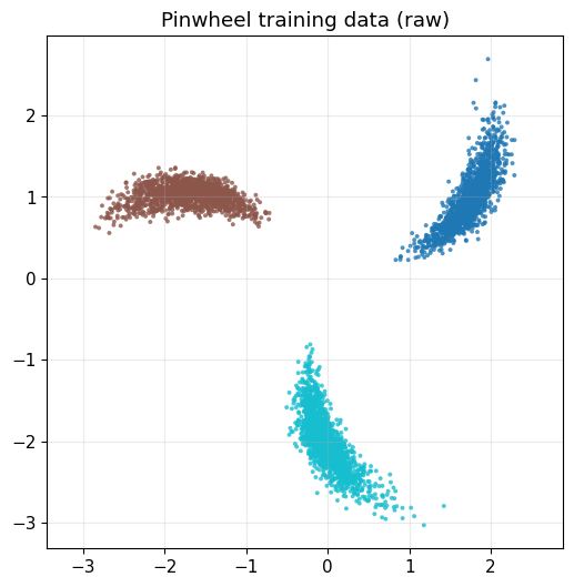
x_train_raw, y_train = make_pinwheel(
    n_samples=4500,
    radial_std=0.18,
    tangential_std=0.06,
    num_classes=3,
    rate=0.18,
    scale=2.0,
    seed=12,
)

plot_dataset_with_labels(x_train_raw, y_train, title="Pinwheel training data (raw)")

x_train, norm_stats = normalize_data(x_train_raw)
# plot_dataset_with_labels(x_train, y_train, title="Pinwheel training data (normalized)")

# ----------------------------
# 2. Diffusion setup
# ----------------------------
T = 100
betas, alphas, alpha_bars = make_linear_beta_schedule(T)

timesteps = np.arange(1, T + 1)
# plt.figure(figsize=(7, 4))
# plt.plot(timesteps, np.sqrt(alpha_bars), label=r'$\sqrt{\bar{\alpha}_t}$')
# plt.plot(timesteps, np.sqrt(1.0 - alpha_bars), label=r'$\sqrt{1-\bar{\alpha}_t}$')
# plt.xlabel("timestep t")
# plt.ylabel("scale")
# plt.title("Forward diffusion signal/noise scales")
# plt.legend()
# plt.grid(True, alpha=0.25)
# plt.show()

# ----------------------------
# 3. Build weaker model
# ----------------------------
model = SmallDenoiserMLP(
    x_dim=2,
    t_dim=24,
    h1=64,
    h2=64,
    seed=0,
)

# ----------------------------
# 4. Train model
# ----------------------------
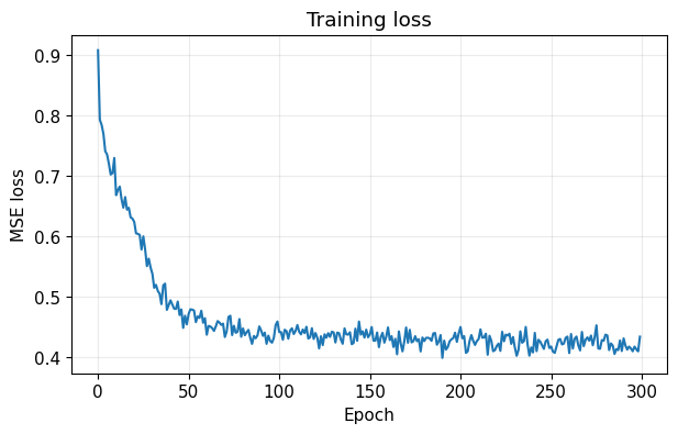
losses = train_ddim_denoiser(
    model=model,
    x_train=x_train,
    T=T,
    alpha_bars=alpha_bars,
    epochs=300,
    batch_size=256,
    lr=1.2e-3,
    lr_decay=0.998,
    grad_clip=1.0,
    seed=42,
    verbose_every=25,
)

plot_training_loss(losses)

# ----------------------------
# 5. DDIM inference: deterministic
# ----------------------------
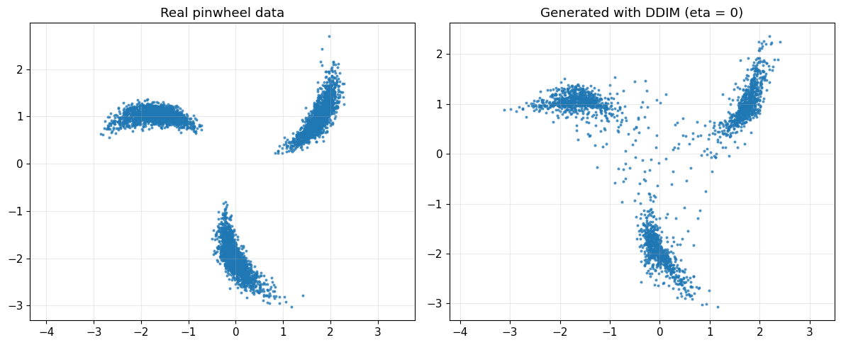
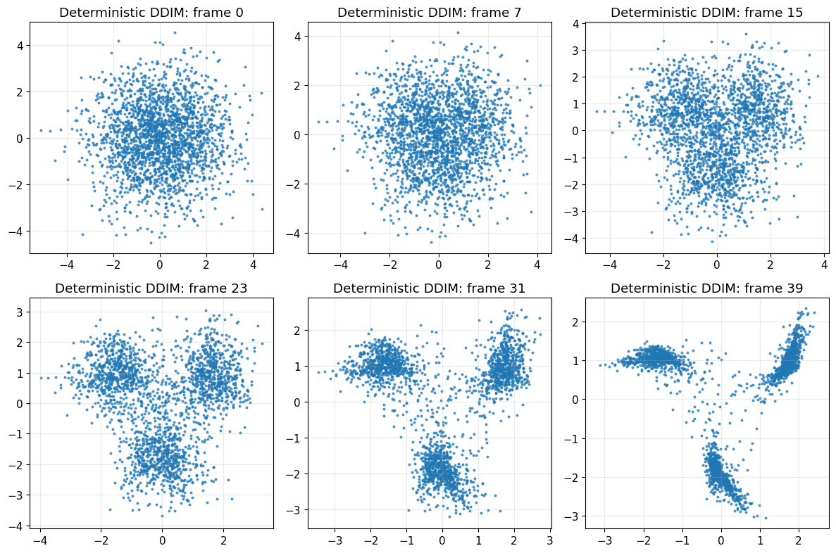
x_gen_det_norm, seq_det, path_det_norm = sample_ddim(
    model=model,
    n_samples=2200,
    T=T,
    alpha_bars=alpha_bars,
    num_steps=40,
    eta=0.0,
    seed=123,
    store_path=True,
)

x_gen_det = denormalize_data(x_gen_det_norm, norm_stats)
path_det = [denormalize_data(x, norm_stats) for x in path_det_norm]

plot_real_vs_generated(
    x_real=x_train_raw,
    x_gen=x_gen_det,
    title_real="Real pinwheel data",
    title_gen="Generated with DDIM (eta = 0)"
)

plot_sampling_path(path_det, title_prefix="Deterministic DDIM")

# ----------------------------
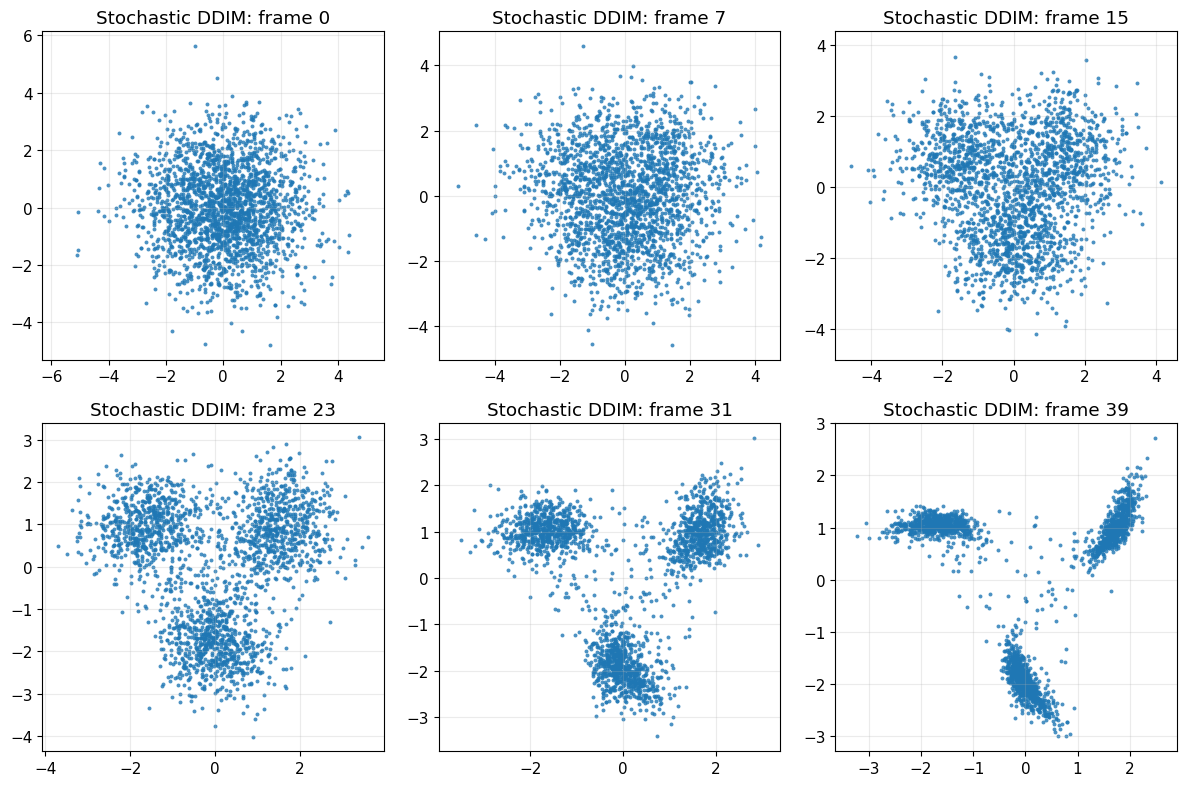
# 6. DDIM inference: stochastic
# ----------------------------
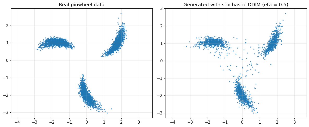
x_gen_sto_norm, seq_sto, path_sto_norm = sample_ddim(
    model=model,
    n_samples=2200,
    T=T,
    alpha_bars=alpha_bars,
    num_steps=40,
    eta=0.5,
    seed=456,
    store_path=True,
)

x_gen_sto = denormalize_data(x_gen_sto_norm, norm_stats)
path_sto = [denormalize_data(x, norm_stats) for x in path_sto_norm]

plot_real_vs_generated(
    x_real=x_train_raw,
    x_gen=x_gen_sto,
    title_real="Real pinwheel data",
    title_gen="Generated with stochastic DDIM (eta = 0.5)"
)

plot_sampling_path(path_sto, title_prefix="Stochastic DDIM")

# ----------------------------
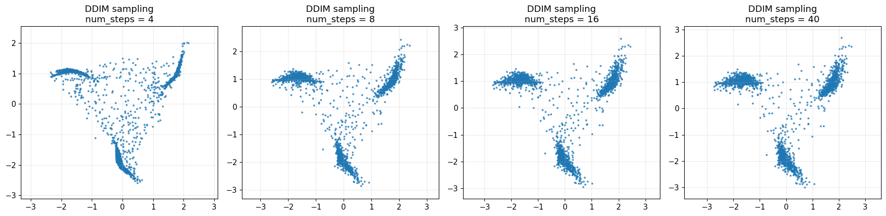
# 7. Compare different DDIM step counts
# ----------------------------
step_choices = [4, 8, 16, 40]
gen_results = []

shared_seed = 999

for num_steps in step_choices:
    x_gen_norm, _, _ = sample_ddim(
        model=model,
        n_samples=1800,
        T=T,
        alpha_bars=alpha_bars,
        num_steps=num_steps,
        eta=0.0,
        seed=shared_seed,
        store_path=False,
    )
    x_gen = denormalize_data(x_gen_norm, norm_stats)
    gen_results.append((num_steps, x_gen))

fig, axes = plt.subplots(1, len(step_choices), figsize=(18, 4.5))
for ax, (num_steps, x_gen) in zip(axes, gen_results):
    ax.scatter(x_gen[:, 0], x_gen[:, 1], s=8, alpha=0.8, linewidths=0)
    ax.set_title(f"DDIM sampling\nnum_steps = {num_steps}")
    ax.axis("equal")
    ax.grid(True, alpha=0.25)

plt.tight_layout()
plt.show()

# ----------------------------
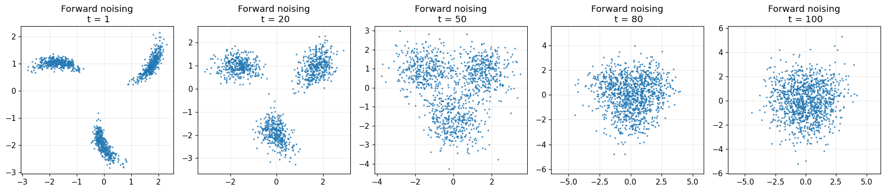
# 8. Show forward corruption examples
# ----------------------------
rng_vis = np.random.default_rng(0)
subset = x_train[:1200]
chosen_t = [1, 20, 50, 80, 100]

fig, axes = plt.subplots(1, len(chosen_t), figsize=(18, 4))
for ax, t in zip(axes, chosen_t):
    t_idx = np.full(len(subset), t, dtype=int)
    x_t_norm, _ = sample_q_xt_given_x0(subset, t_idx, alpha_bars, rng_vis)
    x_t = denormalize_data(x_t_norm, norm_stats)

    ax.scatter(x_t[:, 0], x_t[:, 1], s=6, alpha=0.8, linewidths=0)
    ax.set_title(f"Forward noising\n t = {t}")
    ax.axis("equal")
    ax.grid(True, alpha=0.25)

plt.tight_layout()
plt.show()

Epoch    1 | loss = 0.907566 | lr = 0.001198
Epoch   25 | loss = 0.578273 | lr = 0.001141
Epoch   50 | loss = 0.454475 | lr = 0.001086
Epoch   75 | loss = 0.436877 | lr = 0.001033
Epoch  100 | loss = 0.459271 | lr = 0.000982
Epoch  125 | loss = 0.420282 | lr = 0.000934
Epoch  150 | loss = 0.433237 | lr = 0.000889
Epoch  175 | loss = 0.426662 | lr = 0.000845
Epoch  200 | loss = 0.439302 | lr = 0.000804
Epoch  225 | loss = 0.426611 | lr = 0.000765
Epoch  250 | loss = 0.415550 | lr = 0.000727
Epoch  275 | loss = 0.433010 | lr = 0.000692
Epoch  300 | loss = 0.434203 | lr = 0.000658