Fall 2025 - Diffusion Guest Lecture

Fall 2025 - Diffusion Guest Lecture#

Use the Live Code feature on this page using the icon on top.

Live Code feature works on this page.

Function Approximators#

Neural networks are universal function approximators.
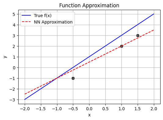
They learn to model an unknown function \(y = f(x)\) by training on pairs of \((x, y)\).

Given data points:

\((1, 2), (1.5, 3), (-0.5, -1)\), a network can learn \(f\) and predict \(y\) for new \(x\).

The goal is to find a function \(f\) such that:

\[ y = f(x) \]

In practice, \(f\) is parameterized by trainable weights.

import numpy as np
import matplotlib.pyplot as plt
from ipywidgets import interact, FloatSlider

# Toggle ON/OFF
interactive = True  # ⇦ SET TO True or False

# True function to approximate
def true_f(x):
    return 2 * x + 1

# Main plotting logic
def plot_approximation(weight=1.5, bias=0.5):
    x = np.linspace(-2, 2, 100)
    y_true = true_f(x)
    y_pred = weight * x + bias

    plt.figure(figsize=(6, 4))
    plt.plot(x, y_true, label='True f(x)', color='blue')
    plt.plot(x, y_pred, label='NN Approximation', linestyle='--', color='red')
    plt.scatter([1, 1.5, -0.5], [2, 3, -1], color='black')
    plt.title('Function Approximation')
    plt.xlabel('x')
    plt.ylabel('y')
    plt.legend()
    plt.grid(True)
    plt.show()

# Interactive or Static
if interactive:
    interact(
        plot_approximation,
        weight=FloatSlider(value=1.5, min=-5, max=5, step=0.1),
        bias=FloatSlider(value=0.5, min=-5, max=5, step=0.1)
    )
else:
    plot_approximation()

../_images/1c72fc5f8c30ea082a084952fa7c9f12fe55568f2780c3726f4b0d631c535e05.png

What is Data Distribution?#

Where does data come from?
Behind any dataset is a hidden data-generating process.

A random experiment (like flipping a coin) defines a random variable \(X\) whose outcomes follow a probability distribution \(p(x)\).

For discrete \(X\):

\[ P(X = x) = \text{Probability that X takes value x} \]

For continuous \(X\):

\[ P(a \leq X \leq b) = \int_{a}^{b} p(x) dx \]

The PDF describes how likely different \(x\) values are.

Gaussian Distribution and Central Limit Theorem#

The Gaussian distribution, also called the Normal distribution, is a fundamental continuous probability distribution with a bell-shaped curve. Its probability density function (PDF) for a scalar random variable \(x\) is:

\[ p(x) = \frac{1}{\sqrt{2\pi \sigma^2}} \exp\left( -\frac{(x - \mu)^2}{2\sigma^2} \right) \]

where:

\(\mu\) is the mean (the center of the distribution)
\(\sigma^2\) is the variance (the spread)

The Gaussian is symmetric about \(\mu\) and is fully described by its first two moments.

Central Limit Theorem (CLT):
The CLT states that the sum (or average) of a large number of independent and identically distributed (i.i.d.) random variables — regardless of their original distribution — will approximate a Gaussian distribution as the number of variables grows large. Formally:

\[ \text{If} \quad X_1, X_2, \dots, X_n \text{ are i.i.d. with mean } \mu \text{ and variance } \sigma^2, \quad \text{then} \quad \frac{1}{n}\sum_{i=1}^n X_i \approx \mathcal{N}\left(\mu, \frac{\sigma^2}{n}\right) \]

The CLT explains why the Gaussian appears so frequently in nature and underpins many generative models and statistical inference techniques.

Why continuous Gaussian estimation is important?#

Sum and Product of Two Gaussians#

Sum of Two Gaussians#

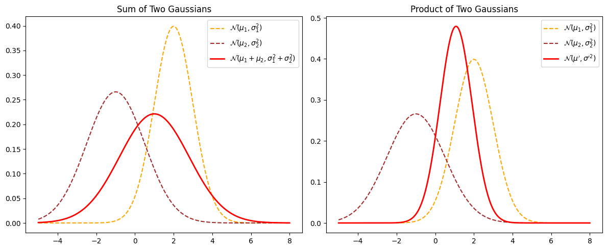
If two random variables \(X\) and \(Y\) are independent and both normally distributed:

\[ X \sim \mathcal{N}(\mu_X, \sigma_X^2), \quad Y \sim \mathcal{N}(\mu_Y, \sigma_Y^2) \]

then their sum \(Z = X + Y\) is also Gaussian:

\[ Z \sim \mathcal{N}(\mu_X + \mu_Y, \; \sigma_X^2 + \sigma_Y^2). \]

The mean adds and the variances add.

Product of Two Gaussians#

If we multiply the PDFs of two Gaussian distributions (often used in Bayesian updating), the result is proportional to another Gaussian:

\[ p(x) \propto \mathcal{N}(x | \mu_1, \sigma_1^2) \times \mathcal{N}(x | \mu_2, \sigma_2^2). \]

The product is:

\[ p(x) = \mathcal{N}\Big( x \;|\; \mu', \sigma'^2 \Big) \]

where:

\[ \sigma'^2 = \left( \frac{1}{\sigma_1^2} + \frac{1}{\sigma_2^2} \right)^{-1}, \quad \mu' = \sigma'^2 \left( \frac{\mu_1}{\sigma_1^2} + \frac{\mu_2}{\sigma_2^2} \right). \]

So the product of two Gaussians is another Gaussian with updated mean and variance.

This property is fundamental for many Bayesian inference and Kalman filter algorithms.

from scipy.stats import norm

# Define parameters for two Gaussian distributions
mu1, sigma1 = 2, 1
mu2, sigma2 = -1, 1.5

# Define the range for plotting
x = np.linspace(-5, 8, 500)

# Compute the PDFs of the two Gaussians
pdf1 = norm.pdf(x, mu1, sigma1)
pdf2 = norm.pdf(x, mu2, sigma2)

# Sum of two independent Gaussians
mu_sum = mu1 + mu2
sigma_sum = np.sqrt(sigma1**2 + sigma2**2)
pdf_sum = norm.pdf(x, mu_sum, sigma_sum)

# Product of two Gaussians (up to a normalization constant)
sigma_prod = np.sqrt((sigma1**2 * sigma2**2) / (sigma1**2 + sigma2**2))
mu_prod = (mu1 * sigma2**2 + mu2 * sigma1**2) / (sigma1**2 + sigma2**2)
pdf_prod = norm.pdf(x, mu_prod, sigma_prod)

# Plot the Gaussians
plt.figure(figsize=(12, 5))

# Subplot for Sum of Gaussians
plt.subplot(1, 2, 1)
plt.plot(x, pdf1, label=r'$\mathcal{N}(\mu_1, \sigma_1^2)$', linestyle='dashed', color='orange')
plt.plot(x, pdf2, label=r'$\mathcal{N}(\mu_2, \sigma_2^2)$', linestyle='dashed', color='brown')
plt.plot(x, pdf_sum, label=r'$\mathcal{N}(\mu_1+\mu_2, \sigma_1^2+\sigma_2^2)$', linewidth=2, color='red')
plt.title('Sum of Two Gaussians')
plt.legend()

# Subplot for Product of Gaussians
plt.subplot(1, 2, 2)
plt.plot(x, pdf1, label=r'$\mathcal{N}(\mu_1, \sigma_1^2)$', linestyle='dashed', color='orange')
plt.plot(x, pdf2, label=r'$\mathcal{N}(\mu_2, \sigma_2^2)$', linestyle='dashed', color='brown')
plt.plot(x, pdf_prod, label=r'$\mathcal{N}(\mu^\prime, \sigma^{\prime 2})$', linewidth=2, color='red')
plt.title('Product of Two Gaussians')
plt.legend()

plt.tight_layout()
plt.show()

../_images/19405c07e710ee7220a9ece9efb95c5c8480b7731cc8efd2361a10b210dfb9e4.png

Expected Value: Definition and Practical Implementation#

The expected value (or mean) is a fundamental concept in probability and statistics that represents the long-run average outcome of a random variable.

For a continuous random variable X with probability density function p(x), the expected value is defined as:

\[ \mathbb{E}[X] = \int_{-\infty}^{\infty} x , p(x) , dx \]

For a discrete random variable:

\[ \mathbb{E}[X] = \sum_{i} x_i , P(X = x_i) \]

When we only have a finite sample x_1, x_2, \(\ldots\), x_n, the expected value is approximated by the sample mean:

\[ \hat{\mu} = \frac{1}{n} \sum_{i=1}^{n} x_i \]

Interpolation as a Simple Generative Technique#

Interpolation is a basic yet powerful concept in generative modeling. When we interpolate, we create new data points by finding values between existing data points.

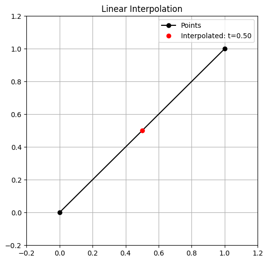
For example, given two data points x_1 and x_2, a simple linear interpolation is:

\[ x_{\text{new}} = (1 - \alpha) , x_1 + \alpha , x_2,\quad \alpha \in [0, 1]. \]

By varying \alpha between 0 and 1, we generate a smooth transition between the two original data points.

Why is this useful? • In low dimensions, it helps to fill gaps between sparse data. • In high-dimensional spaces (like images or embeddings), it is used to smoothly blend features. • Many generative models (e.g., VAEs) use interpolation in latent space to show how well the model captures smooth, meaningful variations in data.

Key idea:

Interpolation doesn’t truly create data from scratch, but it extends the dataset by exploiting the structure of known points. It’s a simple starting point for understanding how generative models synthesize new samples.

import numpy as np
import matplotlib.pyplot as plt
from ipywidgets import interact, FloatSlider

interactive = True

def plot_interpolation(t=0.5):
    p0 = np.array([0, 0])
    p1 = np.array([1, 1])
    p = (1 - t) * p0 + t * p1

    plt.figure(figsize=(6, 6))
    plt.plot([p0[0], p1[0]], [p0[1], p1[1]], 'ko-', label='Points')
    plt.plot(p[0], p[1], 'ro', label=f'Interpolated: t={t:.2f}')
    plt.title("Linear Interpolation")
    plt.xlim(-0.2, 1.2)
    plt.ylim(-0.2, 1.2)
    plt.grid(True)
    plt.legend()
    plt.show()

if interactive:
    interact(
        plot_interpolation,
        t=FloatSlider(value=0.5, min=0.0, max=1.0, step=0.01)
    )
else:
    plot_interpolation()

../_images/eb422a6b95d8d0b99e79a9c19812931c84da3090e5669630d409f89e993d093a.png

Multivariate Gaussian Distribution#

A multivariate Gaussian distribution generalizes the normal distribution to multiple dimensions.
It models a vector of random variables \(\mathbf{X} \in \mathbb{R}^d\) that are jointly Gaussian.

Probability Density Function (PDF)#

The PDF of a \(d\)-dimensional multivariate Gaussian is:

\[ p(\mathbf{x}) = \frac{1}{(2\pi)^{d/2} |\boldsymbol{\Sigma}|^{1/2}} \exp \left( - \frac{1}{2} (\mathbf{x} - \boldsymbol{\mu})^T \boldsymbol{\Sigma}^{-1} (\mathbf{x} - \boldsymbol{\mu}) \right) \]

where:

\(\mathbf{x} \in \mathbb{R}^d\) is the data vector,
\(\boldsymbol{\mu} \in \mathbb{R}^d\) is the mean vector,
\(\boldsymbol{\Sigma} \in \mathbb{R}^{d \times d}\) is the covariance matrix,
\(|\boldsymbol{\Sigma}|\) denotes the determinant of the covariance matrix,
\(\boldsymbol{\Sigma}^{-1}\) is its inverse.

Key Properties#

The mean vector \(\boldsymbol{\mu}\) defines the center of the distribution.
The covariance matrix \(\boldsymbol{\Sigma}\) encodes the variance of each dimension and the correlations between dimensions.
If variables are uncorrelated, \(\boldsymbol{\Sigma}\) is diagonal.

The multivariate Gaussian is fundamental for modeling high-dimensional continuous data and is widely used in generative modeling, probabilistic PCA, and Bayesian statistics.

t-SNE: How It Works & How This Code Implements It#

What is t-SNE?

t-SNE (t-Distributed Stochastic Neighbor Embedding) is a nonlinear dimensionality reduction technique for visualizing high-dimensional data in 2D or 3D.
It preserves local structure: points close in high-dimensional space remain close in the low-dimensional map.
It works by converting pairwise distances into probability distributions:
- In the high-dimensional space, similar points have higher conditional probability of being neighbors.
- In the low-dimensional map, a similar distribution is constructed.
- The algorithm minimizes the Kullback-Leibler (KL) divergence between these two distributions.

Key Steps in t-SNE

Compute pairwise distances

Uses squared Euclidean distance.

Convert distances to probabilities

High-dimensional distances → conditional probabilities via a Gaussian kernel.
Each point’s bandwidth (sigma) is found via binary search so its perplexity matches the target value (controls effective neighborhood size).

Map to low dimensions

Points are initialized randomly in 2D.
Gradient descent adjusts positions to match the high- and low-dimensional probability distributions.

Symmetrize probabilities

Conditional probabilities are symmetrized to form joint probabilities.

Cost function

KL divergence measures how well the low-dimensional map matches the high-dimensional similarities.

How This Code Implements It

neg_squared_euc_dists — Computes negative squared Euclidean distances between points.

find_optimal_sigmas + binary_search — Finds the best sigma for each point to match the target perplexity.

p_joint — Computes the high-dimensional joint probability matrix.

q_tsne or q_joint — Computes the low-dimensional probability matrix (uses Student-t kernel for t-SNE).

estimate_sne — Runs gradient descent to adjust the embedding.

tsne_grad or symmetric_sne_grad — Computes the gradient of the cost function.

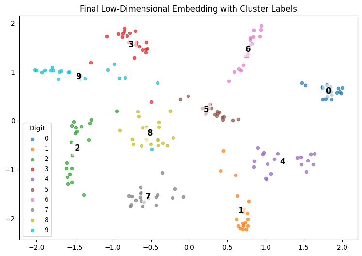
plot_embedding — Plots the final 2D embedding and labels each cluster at its mean.

Result:
This notebook loads digit data, computes a meaningful 2D embedding with t-SNE or SNE, and plots all classes clearly labeled at their cluster centers.

Show code cell source

Hide code cell source

import numpy as np
import matplotlib.pyplot as plt
from sklearn.datasets import load_digits

def neg_squared_euc_dists(X):
    sum_X = np.sum(np.square(X), 1)
    D = np.add(np.add(-2 * np.dot(X, X.T), sum_X).T, sum_X)
    return -D

def softmax(X, diag_zero=True):
    e_x = np.exp(X - np.max(X, axis=1).reshape([-1, 1]))
    if diag_zero:
        np.fill_diagonal(e_x, 0.)
    e_x = e_x + 1e-8
    return e_x / e_x.sum(axis=1).reshape([-1, 1])

def calc_prob_matrix(distances, sigmas=None):
    if sigmas is not None:
        two_sig_sq = 2. * np.square(sigmas.reshape((-1, 1)))
        return softmax(distances / two_sig_sq)
    else:
        return softmax(distances)

def binary_search(eval_fn, target, tol=1e-10, max_iter=10000, lower=1e-20, upper=1000.):
    for _ in range(max_iter):
        guess = (lower + upper) / 2.
        val = eval_fn(guess)
        if val > target:
            upper = guess
        else:
            lower = guess
        if np.abs(val - target) <= tol:
            break
    return guess

def calc_perplexity(prob_matrix):
    entropy = -np.sum(prob_matrix * np.log2(prob_matrix), 1)
    perplexity = 2 ** entropy
    return perplexity

def perplexity(distances, sigmas):
    return calc_perplexity(calc_prob_matrix(distances, sigmas))

def find_optimal_sigmas(distances, target_perplexity):
    sigmas = []
    for i in range(distances.shape[0]):
        eval_fn = lambda sigma: perplexity(distances[i:i+1, :], np.array(sigma))
        correct_sigma = binary_search(eval_fn, target_perplexity)
        sigmas.append(correct_sigma)
    return np.array(sigmas)

def q_joint(Y):
    distances = neg_squared_euc_dists(Y)
    exp_distances = np.exp(distances)
    np.fill_diagonal(exp_distances, 0.)
    return exp_distances / np.sum(exp_distances), None

def p_conditional_to_joint(P):
    return (P + P.T) / (2. * P.shape[0])

def p_joint(X, target_perplexity):
    distances = neg_squared_euc_dists(X)
    sigmas = find_optimal_sigmas(distances, target_perplexity)
    p_conditional = calc_prob_matrix(distances, sigmas)
    P = p_conditional_to_joint(p_conditional)
    return P

def symmetric_sne_grad(P, Q, Y, _):
    pq_diff = P - Q
    pq_expanded = np.expand_dims(pq_diff, 2)
    y_diffs = np.expand_dims(Y, 1) - np.expand_dims(Y, 0)
    grad = 4. * (pq_expanded * y_diffs).sum(1)
    return grad

def tsne_grad(P, Q, Y, inv_distances):
    pq_diff = P - Q
    pq_expanded = np.expand_dims(pq_diff, 2)
    y_diffs = np.expand_dims(Y, 1) - np.expand_dims(Y, 0)
    distances_expanded = np.expand_dims(inv_distances, 2)
    y_diffs_wt = y_diffs * distances_expanded
    grad = 4. * (pq_expanded * y_diffs_wt).sum(1)
    return grad

def q_tsne(Y):
    distances = neg_squared_euc_dists(Y)
    inv_distances = 1. / (1. - distances)
    np.fill_diagonal(inv_distances, 0.)
    Q = inv_distances / np.sum(inv_distances)
    return Q, inv_distances

def estimate_sne(X, P, rng, num_iters, q_fn, grad_fn, learning_rate, momentum):
    Y = rng.normal(0., 0.0001, [X.shape[0], 2])
    if momentum:
        Y_m2 = Y.copy()
        Y_m1 = Y.copy()
    for _ in range(num_iters):
        Q, distances = q_fn(Y)
        grads = grad_fn(P, Q, Y, distances)
        Y = Y - learning_rate * grads
        if momentum:
            Y += momentum * (Y_m1 - Y_m2)
            Y_m2 = Y_m1.copy()
            Y_m1 = Y.copy()
    return Y

def plot_embedding(Y, labels, figsize=(9, 6)):
    plt.figure(figsize=figsize)
    classes = np.unique(labels)
    for label in classes:
        idx = labels == label
        plt.scatter(Y[idx, 0], Y[idx, 1], label=str(label), alpha=0.7, s=20)
        # Add text label at cluster mean
        mean_x, mean_y = Y[idx, 0].mean(), Y[idx, 1].mean()
        plt.text(mean_x, mean_y, str(label), fontsize=12, weight='bold',
                 ha='center', va='center', color='black',
                 bbox=dict(facecolor='white', alpha=0.6, edgecolor='none'))
    plt.legend(title="Digit")
    plt.title("Final Low-Dimensional Embedding with Cluster Labels")
    plt.show()

../_images/0ed5b78ce5d2d67c9d26db549701d18d0af6dd868967198933738d335c4ce48a.png

Encoder Decoder models for Data Generation#

Diffusion Models#

1. Motivation and Recap#

VAEs and GANs both aim to model complex data distributions.
VAEs: reconstruct well but can produce blurry samples due to simplified likelihood assumptions.
GANs: generate sharp samples but training can be unstable (mode collapse, convergence issues).

Diffusion Models offer a new paradigm:

They learn to generate data by gradually denoising a noisy input, reversing a diffusion (noise) process.
State-of-the-art in generative modeling, powering modern tools like Stable Diffusion and DALL·E 2.

2. Diffusion Models: Core Idea#

A diffusion model defines two processes:

Forward Diffusion Process (noising):
Gradually adds Gaussian noise to data \( \mathbf{x}_0 \) over \( T \) steps until it becomes nearly pure noise \( \mathbf{x}_T \).
Reverse Diffusion Process (denoising):
Learns to reverse the noising step-by-step, generating realistic samples from noise.

3. Forward Diffusion Process#

We start with data sample \( \mathbf{x}_0 \sim q(\mathbf{x}_0) \).
Noise is added in small steps controlled by a variance schedule \( \{\beta_t\}_{t=1}^T \), where \( \beta_t \in (0,1) \).

3.1 Single Step#

\[ q(\mathbf{x}_t \mid \mathbf{x}_{t-1}) = \mathcal{N}\!\left( \sqrt{1 - \beta_t}\,\mathbf{x}_{t-1}, \, \beta_t \mathbf{I} \right) \]

3.2 Closed-Form Sampling#

We can directly sample \( \mathbf{x}_t \) at step \( t \) from \( \mathbf{x}_0 \):

\[ q(\mathbf{x}_t \mid \mathbf{x}_0) = \mathcal{N}\!\left( \sqrt{\bar{\alpha}_t}\, \mathbf{x}_0, \, (1-\bar{\alpha}_t)\mathbf{I} \right) \]

where:

\[ \alpha_t = 1 - \beta_t, \quad \bar{\alpha}_t = \prod_{s=1}^t \alpha_s \]

and noise injection is:

\[ \mathbf{x}_t = \sqrt{\bar{\alpha}_t}\,\mathbf{x}_0 + \sqrt{1-\bar{\alpha}_t}\,\boldsymbol{\epsilon}, \quad \boldsymbol{\epsilon} \sim \mathcal{N}(0,I) \]

4. Reverse Diffusion Process#

We want to reverse the noising process:

\[ p_{\theta}(\mathbf{x}_{t-1} \mid \mathbf{x}_t) = \mathcal{N}\!\left(\mu_{\theta}(\mathbf{x}_t, t), \, \Sigma_{\theta}(\mathbf{x}_t, t)\right) \]

The reverse conditionals are also Gaussian but unknown.
A neural network (usually a U-Net) is trained to predict the mean (and sometimes variance).

In practice, instead of directly predicting \( \mu \), we train the network to predict the noise \( \boldsymbol{\epsilon} \) added at each step.

5. Diffusion Model Training Objective#

Using variational inference, the training objective reduces to:

\[ \mathcal{L}_{\text{diffusion}} = \mathbb{E}_{t, \mathbf{x}_0, \boldsymbol{\epsilon}} \left[ \big\| \boldsymbol{\epsilon} - \boldsymbol{\epsilon}_{\theta}(\mathbf{x}_t, t) \big\|^2 \right] \]

Here, \( \boldsymbol{\epsilon} \) is the true Gaussian noise,
\( \boldsymbol{\epsilon}_{\theta} \) is the predicted noise by the network.

Thus, the network learns to denoise step by step.

6. Comparison: VAEs vs Diffusion Models#

VAE Loss:

\[ \mathcal{L}_{\text{VAE}} = \text{Reconstruction Loss} + \text{KL Divergence} \]

Diffusion Loss:

\[ \mathcal{L}_{\text{Diffusion}} = \text{Noise Matching (MSE between true and predicted noise)} \]

Diffusion models avoid blurry reconstructions by directly learning the data distribution via noise prediction.

Fall 2025 - Diffusion Guest Lecture

Contents

Fall 2025 - Diffusion Guest Lecture#

Function Approximators#

What is Data Distribution?#

Gaussian Distribution and Central Limit Theorem#

Why continuous Gaussian estimation is important?#

Sum and Product of Two Gaussians#

Sum of Two Gaussians#

Product of Two Gaussians#

Expected Value: Definition and Practical Implementation#

Interpolation as a Simple Generative Technique#

Multivariate Gaussian Distribution#

Probability Density Function (PDF)#

Key Properties#

t-SNE: How It Works & How This Code Implements It#

Encoder Decoder models for Data Generation#

Diffusion Models#

1. Motivation and Recap#

2. Diffusion Models: Core Idea#

3. Forward Diffusion Process#

3.1 Single Step#

3.2 Closed-Form Sampling#

4. Reverse Diffusion Process#

5. Diffusion Model Training Objective#

6. Comparison: VAEs vs Diffusion Models#

Forward Diffusion Interactive Animation#

Reverse Diffusion Interactive Animation#

Forward and Reverse Diffusion on Images#