Convolutional Neural Networks from Scratch with Live Code

Convolutional Neural Networks from Scratch with Live Code#

In this lecture, we will discuss Convolutional Neural Networks in detail and code a CNN model from scratch. Students shall also have the ability to utilize the “Live Code” feature in this website to interact with python code for in-depth understanding.

What is an Image?#

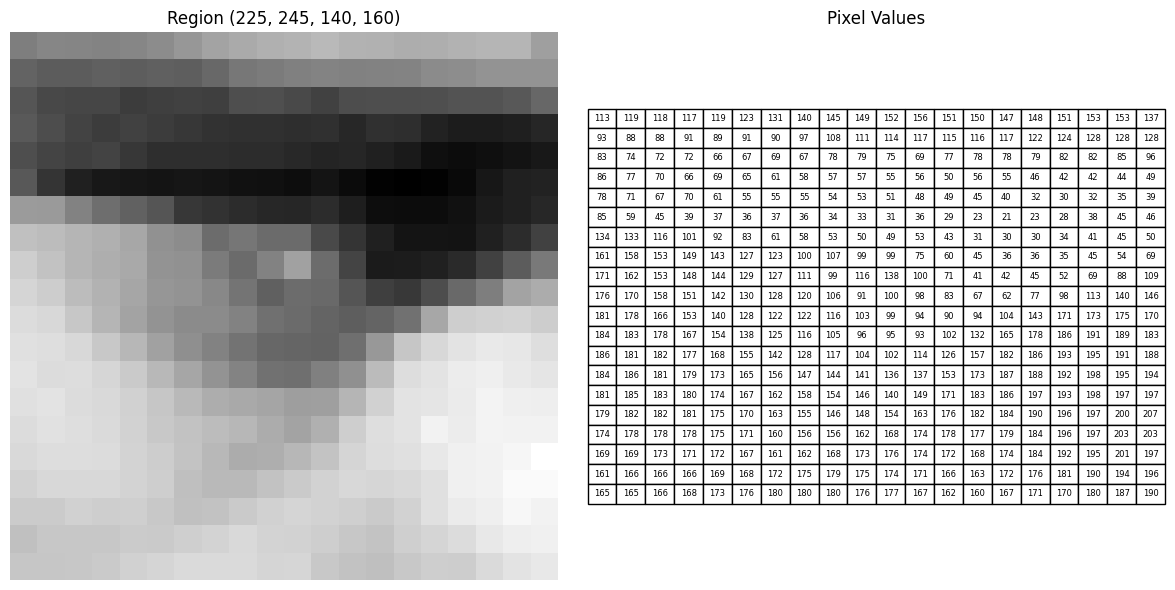
An image is made up of a grid of tiny squares called pixels. Each pixel holds a bit of color and brightness, and when you put them all together, they form the full picture you see. For grayscale images, each pixel holds intensity values that range from \(0\) to \(255\). Matplotlib is a nice tool to plot images on 2D axes.

Let’s explore and learn more about images.

# Camera is a grayscale image from skimage
img = camera().astype(np.float32) # example image

plt.figure(figsize=(4, 4))
plt.imshow(img, cmap="gray")
plt.title(f"Image Shape: {img.shape}") 
plt.show()

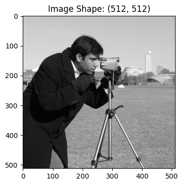
../_images/7a01bbf2d88ebbae49041e44409f404727d0ad25b1170da4c9728bd2a64102e8.png

In the above plot, we see an example image of shape \((512, 512)\). This denotes that the image is a grayscale image (2-dimensional). If we take a closer look at some regions of the image we see that each pixel contains intensity values from \(0\) to \(255\).

../_images/877422c71963cbaa65e988b33ccf4c709576064ccaa538d6220ea0bca99299fd.png

Recap of a Convolution Operation on an Image#

Convolution is an operation that “slides” a small kernel \(K\) over an image \(I\). At each location \((i,j)\), you take a weighted sum of the pixels under the kernel to produce the output pixel \(O(i,j)\).

Discrete Formula#

\[ I \in \mathbb{R}^{H \times W}, \quad K \in \mathbb{R}^{(2r+1) \times (2r+1)}, \quad r = \frac{k-1}{2}. \]

The convolution \(O = I * K\) is defined by

\[ O(i,j) = \sum_{u=-r}^{r} \sum_{v=-r}^{r} I\bigl(i+u,\,j+v\bigr)\;K\bigl(-u,\,-v\bigr), \]

for \(i = 0, \dots, H-1\) and \(j = 0, \dots, W-1\).

Note: The indices \((-u,-v)\) indicate that the kernel is flipped both horizontally and vertically.

Why Flip the Kernel?

Mathematical Consistency
Flipping makes convolution commutative:

\[ I * K = K * I, \]

which is important for many theoretical results (e.g., convolution theorems in Fourier analysis).
System Response Interpretation
In signal processing, convolution represents the response of a system with impulse response \(K\). Flipping aligns the “past” and “future” contributions correctly.
Distinction from Cross-Correlation
If you omit the flip and write

\[ \sum_{u=-r}^{r} \sum_{v=-r}^{r} I(i+u,\,j+v)\;K(u,v), \]

you get cross-correlation instead of convolution. Cross-correlation measures similarity, while convolution implements filtering.

Putting it all together, the flip ensures both the desired mathematical properties (commutativity, associativity) and the correct interpretation of the kernel as an impulse response.

Convolution with Stride and Padding

Convolution with Stride and Padding

\[ I \in \mathbb{R}^{H \times W}, \quad K \in \mathbb{R}^{k \times k}, \quad s \in \mathbb{N} \ (\text{stride}), \quad p \in \mathbb{N} \ (\text{padding}). \]

Padded Image

We surround \(I\) with a border of \(p\) zeros on all sides to form
\(I_{\text{pad}} \in \mathbb{R}^{(H+2p) \times (W+2p)}\), defined by

\[\begin{split} I_{\text{pad}}(x,y) = \begin{cases} I(x - p,\, y - p), & \text{if } 0 \leq x - p < H,\; 0 \leq y - p < W, \\ 0, & \text{otherwise}. \end{cases} \end{split}\]

Output Dimensions

The output \(O \in \mathbb{R}^{H_{\text{out}} \times W_{\text{out}}}\) has

\[ H_{\text{out}} = \left\lfloor \frac{H + 2p - k}{s} \right\rfloor + 1, \quad W_{\text{out}} = \left\lfloor \frac{W + 2p - k}{s} \right\rfloor + 1. \]

Convolution Operation

Slide \(K\) in steps of \(s\) over \(I_{\text{pad}}\):

\[ O(i,j) = \sum_{u=0}^{k-1} \sum_{v=0}^{k-1} I_{\text{pad}}(i \times s + u,\, j \times s + v) \times K(u,v), \]

for \(i = 0, \dots, H_{\text{out}}-1\) and \(j = 0, \dots, W_{\text{out}}-1\).

Why These Matter
Stride \(s\):
Controls how far the kernel jumps each time.
- \(s=1\): full resolution
- \(s>1\): downsampling (reduces output size and computation)
Padding \(p\):
Includes border pixels and controls output size.
- \(p=0\): no padding (shrinks output)
- \(p = \frac{k-1}{2}\) (for odd \(k\)): preserves input size (“same” convolution).

https://upload.wikimedia.org/wikipedia/commons/1/19/2D_Convolution_Animation.gif — Fig. 3 Convolution Example#

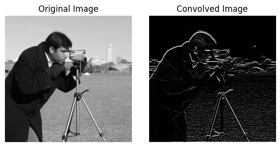
Convolution on 2D images Code#

Test with different kernels to understand what features are extracted by convolution operations.

Show code cell source Hide code cell source

def pad_image(image, padding):
    """
    Zero-pad a 2D image.
    """
    return np.pad(image, pad_width=padding, mode='constant', constant_values=0)

def convolve2d(image, kernel, stride=1, padding=0):
    """
    Perform 2D convolution with optional stride and zero-padding.

    Args:
        image (np.ndarray): Grayscale image (H x W)
        kernel (np.ndarray): Convolution kernel (k x k)
        stride (int): Stride for sliding the kernel
        padding (int): Zero-padding size

    Returns:
        np.ndarray: Convolved output image
    """
    # Flip the kernel for convolution (not needed for cross-correlation)
    kernel = np.flipud(np.fliplr(kernel))

    # Pad the image
    if padding > 0:
        image = pad_image(image, padding)

    H, W = image.shape
    kH, kW = kernel.shape

    # Compute output dimensions
    out_H = (H - kH) // stride + 1
    out_W = (W - kW) // stride + 1

    # Initialize output
    output = np.zeros((out_H, out_W), dtype=np.float32)

    # Perform convolution
    for i in range(out_H):
        for j in range(out_W):
            region = image[i*stride:i*stride+kH, j*stride:j*stride+kW]
            output[i, j] = np.sum(region * kernel)

    # Normalize output to range [0, 255] for display
    output = np.clip(output, 0, 255)

    return output

# 1. Identity (no change)
identity_kernel = np.array([
    [0, 0, 0],
    [0, 1, 0],
    [0, 0, 0]
], dtype=np.float32)

# 2. Simple blur (average)
blur_kernel = np.ones((3, 3), dtype=np.float32) / 9.0

# 3. Gaussian blur
gaussian_blur_kernel = np.array([
    [1, 2, 1],
    [2, 4, 2],
    [1, 2, 1]
], dtype=np.float32) / 16.0

# 4. Sharpen
sharpen_kernel = np.array([
    [0, -1, 0],
    [-1, 5, -1],
    [0, -1, 0]
], dtype=np.float32)

# 5. Edge detection (Sobel X)
sobel_x_kernel = np.array([
    [-1, 0, 1],
    [-2, 0, 2],
    [-1, 0, 1]
], dtype=np.float32)

# 6. Edge detection (Sobel Y)
sobel_y_kernel = np.array([
    [-1, -2, -1],
    [0, 0, 0],
    [1, 2, 1]
], dtype=np.float32)

# 7. Laplacian (strong edge detection)
laplacian_kernel = np.array([
    [0, -1, 0],
    [-1, 4, -1],
    [0, -1, 0]
], dtype=np.float32)

# 8. Emboss
emboss_kernel = np.array([
    [-2, -1, 0],
    [-1, 1, 1],
    [0, 1, 2]
], dtype=np.float32)

# 9. Outline
outline_kernel = np.array([
    [-1, -1, -1],
    [-1, 8, -1],
    [-1, -1, -1]
], dtype=np.float32)

# 10. Box edge (another edge detector)
box_edge_kernel = np.array([
    [1, 1, 1],
    [1, -8, 1],
    [1, 1, 1]
], dtype=np.float32)

# Define kernel
kernel = sobel_y_kernel

# kernel = np.ones((5, 5), dtype=np.float32) / 9.0

# Apply convolution
convolved_img = convolve2d(img, kernel, stride=1, padding=1)  # padding=1 to preserve size

plot_images_grid([img, convolved_img], titles=["Original Image", "Convolved Image"], images_per_row=2, figsize=(6, 3), cmap = "gray")

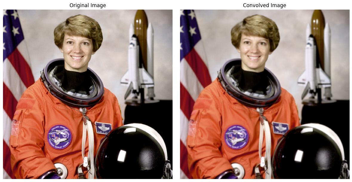
../_images/9d1084c797ec0f1af3e414935d4deac4dcc91d9d867c7b529311053cbaa32814.png

Convolution on RGB images#

from skimage.data import astronaut # RGB image
img_rgb = astronaut().astype(np.float32)

# Example: simple 3D blur kernel
blur_kernel = np.ones((3, 3), dtype=np.float32) / 9.0

out_rgb = convolve3d_custom(img_rgb, blur_kernel)

plot_images_grid([img_rgb.astype(np.uint8), out_rgb], titles=["Original Image", "Convolved Image"], images_per_row=2, figsize=(12, 6))

../_images/6145ae57654be48a3bb5bd93d3408ff2613b96a0dff49170fa6fad28bc27ae5a.png

An image is a function?#

Fourier Transform for Images - Motivation and Foundations

How to View an Image in Fourier Space

A grayscale image is simply a 2D function:

\[ I(x, y) \quad \text{where} \quad (x, y) \in [0, H-1] \times [0, W-1]. \]

It tells you the brightness at each pixel location.

However, instead of thinking pixel-by-pixel,
you can think of an image as a combination of waves of different frequencies.

Each image can be broken down into a sum of sinusoidal waves with different:

Frequencies
Orientations
Amplitudes
Phases

This “alternate view” is called the Fourier space.

What is the 2D Fourier Transform?

The 2D Discrete Fourier Transform (DFT) of an image \(I(x, y)\) is defined as:

\[ F(u, v) = \sum_{x=0}^{H-1} \sum_{y=0}^{W-1} I(x, y)\; e^{-2\pi i \left( \frac{ux}{H} + \frac{vy}{W} \right)}, \]

where:

\(F(u, v)\) tells you how much of the frequency (u, v) exists in the image,
\(i = \sqrt{-1}\) is the imaginary unit,
\(u, v\) represent frequencies (not spatial positions).

What Does the Fourier Transform Give?

Magnitude \(|F(u, v)|\):
Strength (energy) of that frequency component.
Phase \(\arg(F(u, v))\):
Alignment (offset) of that frequency component.

Thus, Fourier space contains two important pieces:

What frequencies are present (magnitude)
How they are arranged (phase)

Why Move to Fourier Space?

Low frequencies correspond to smooth regions (e.g., sky, walls).
High frequencies correspond to edges, textures, sharp changes.

Fourier space lets you:

Analyze or modify an image based on frequency content.
Design filters (like blur, sharpen) more precisely.
Perform fast convolution (because convolution becomes multiplication in Fourier domain).

Inverse Fourier Transform

You can reconstruct the original image from its Fourier coefficients:

\[ I(x, y) = \frac{1}{HW} \sum_{u=0}^{H-1} \sum_{v=0}^{W-1} F(u, v)\; e^{2\pi i \left( \frac{ux}{H} + \frac{vy}{W} \right)}. \]

Thus, Fourier Transform and Inverse Fourier Transform are perfect inverses of each other.

Key Insights

Spatial Domain (Image)	Fourier Domain (Frequency)
Pixel-by-pixel intensity	Waves of different frequencies
Edges, shapes, textures	High-frequency components
Smooth, flat regions	Low-frequency components
Convolution is heavy (slow)	Multiplication is fast

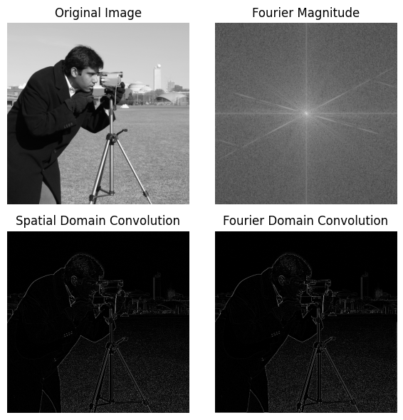
../_images/a18305a8fd031a3c2116dd54598e1bc5a31ffa27ce7c55cbadeaf4932892651d.png

How fast is Fourier Convolution?#

convolve2d time:   4.24693 seconds
fftconvolve time:  0.01665 seconds
Time gain (conv2d / fft): 255.12x
Outputs match? True

Neural Networks as Function Approximators#

At a high level, neural networks are simply function approximators.

They take in data points like \(x_1, x_2, \dots, x_n\) (usually represented as tensors) and learn to predict the corresponding labels \(y_1, y_2, \dots, y_n\).

Formally, a neural network tries to approximate a mapping:

\[ f_\theta(x) \approx y, \]

where:

\(x\) is the input,
\(y\) is the target output,
\(f_\theta\) is the neural network, parameterized by weights \(\theta\),
Learning is the process of adjusting \(\theta\) to minimize the prediction error.

Two Main Components of a Neural Network#

A neural network is generally composed of two main parts:

Feature Extractor Module
- This part processes raw input data into useful internal representations.
- It can be a series of convolutional layers (in images), RNNs (for sequences), or just dense layers.
- Good feature extraction makes the next step easier.
Task-Specific Head
- This part uses the extracted features to solve a specific task.
- Example tasks include classification, regression, segmentation, etc.
- Often consists of one or more fully connected (dense) layers.

Quick Example: TensorFlow Playground#

To visualize this, we can take a look at the TensorFlow Playground.

On this website:

You can see how neural networks learn to extract features from the input space.
You can observe how different architectures affect learning and decision boundaries.
You can interactively modify network shape, learning rates, and visualize how the model improves over time.

Visual Representation of a Simple Neural Network#

Below is a simple diagram showing a basic feedforward neural network:

Understanding Feature Extraction in Convolutional Neural Networks (CNNs)#

1. Intuition: How CNNs Extract Features#

In traditional fully connected networks (MLPs), every neuron is connected to every pixel.
However, in images, nearby pixels are more related than distant pixels.
Thus, local patterns such as edges, textures, and simple shapes are critical to understand an image.

Convolutional Neural Networks (CNNs) use small filters (kernels) that slide across the image and detect these local patterns.

Each filter focuses on extracting specific features such as:

Edges
Corners
Blobs
Textures

These extracted local patterns are organized into feature maps.

2. Mathematical Definition of Convolution in CNNs#

Given:

Input image \(I \in \mathbb{R}^{H \times W}\),
Convolutional kernel \(K \in \mathbb{R}^{k \times k}\),
Stride \(s\),
Padding \(p\),

the output feature map \(O \in \mathbb{R}^{H_{\text{out}} \times W_{\text{out}}}\) is computed as:

\[ O(i, j) = \sum_{u=0}^{k-1} \sum_{v=0}^{k-1} I(i \times s + u, j \times s + v) \cdot K(u, v) \]

where:

\[ H_{\text{out}} = \left\lfloor \frac{H + 2p - k}{s} \right\rfloor + 1, \quad W_{\text{out}} = \left\lfloor \frac{W + 2p - k}{s} \right\rfloor + 1 \]

At each position, the kernel computes a weighted sum over a small patch of the input image, producing one output pixel.

3. Where Are Features Learned?#

The convolutional kernels themselves are learned during training through backpropagation.
Initially, the filters are random. As training progresses, the network updates the kernel weights to detect important patterns that help minimize classification error.

Each output channel in a convolutional layer corresponds to a different feature map, detected by a different kernel.
Thus:

Each kernel learns to recognize a specific pattern.
The number of output channels is equal to the number of filters.

For example:

1 input channel (grayscale image),
32 filters,

results in an output with 32 learned feature maps.

Features are stored and represented across the multiple channels.

4. Why Max Pooling?#

After convolution, the feature maps still contain a lot of redundant information, including slight variations or small shifts.
Max pooling helps by:

Keeping only the strongest activations (important features),
Making the network more robust to small translations or distortions,
Reducing the spatial size of the feature maps, thus reducing computation and parameters.

Max Pooling Operation#

Given a pooling window of size \(p \times p\),
for each window, the output is the maximum value:

\[ O(i, j) = \max_{(u,v) \in p \times p \text{ window}} I(u,v) \]

For example, for a \(2 \times 2\) pooling:

2×2 Window	Max Pool
1 3
2 4	→ 4

Only the maximum value (4) is retained.

5. Overall Flow of a CNN Layer#

Step	Action
Convolution	Detect local patterns using small kernels
Activation (ReLU)	Introduce non-linearity
Max Pooling	Downsample feature maps and focus on important features
Repeat	Stack multiple layers to build increasingly complex representations

6. Summary#

CNNs extract hierarchical features from images.
Convolutional kernels are learned automatically during training.
Each output channel corresponds to a different learned feature map.
Max pooling improves translation invariance and reduces redundancy.
Stacking multiple convolution and pooling layers allows the network to detect edges at first, then textures, and finally complex structures or objects.

Convolutional Neural Networks from Scratch with Live Code

Contents

Convolutional Neural Networks from Scratch with Live Code#

What is an Image?#

Recap of a Convolution Operation on an Image#

Discrete Formula#

Convolution on 2D images Code#

Convolution on RGB images#

An image is a function?#

How fast is Fourier Convolution?#

Neural Networks as Function Approximators#

Two Main Components of a Neural Network#

Quick Example: TensorFlow Playground#

Visual Representation of a Simple Neural Network#

Understanding Feature Extraction in Convolutional Neural Networks (CNNs)#

1. Intuition: How CNNs Extract Features#

2. Mathematical Definition of Convolution in CNNs#

3. Where Are Features Learned?#

4. Why Max Pooling?#

Max Pooling Operation#

5. Overall Flow of a CNN Layer#

6. Summary#